Most companies require rolling forecast input forms that display actual data in read mode and forecast data in write mode. Because this process is repeated each month, it is also a requirement to automatically determine the current month for the user and then format prior versus future months separately. I use a property of the category members (such as ACTUAL or FCST_AUG) to drive the formatting for actual versus forecast data for a low-maintenance solution that automatically locks the actual months for data entry and highlights the forecast months to allow data entry. The master data can then remain the same from month to month.

The benefit is that you can read and write into the same input form that is automatically adjusted each time the next month arrives.

This is an SAP Business Planning and Consolidation (BPC) version 10.0 scenario. SAP BPC version 10.0 uses the Excel SAP Enterprise Performance Management (EPM) add-in. Now I list the steps that you need to take:

1. Use Excel functions to automatically determine the current month and year
2. Use the EPMMemberOffset function to determine the prior and future months
3. Use the EPMMemberProperty function to determine the category ID based on the current month
4. Create a new report with accounts in the rows and time/category in the columns (Note: the sheet option is set to Use as Input Form, which means that the report can be used for both reading and writing.)
5. Change the EPMOlapMember function to bring the current year, month, and category into the EPM report
6. Set up a category dimension property to be used for the formatting
7. Format actual months to be locked for data input and forecast months to data input

Before walking you through these steps, I briefly explain how EPM reports work. When you create an EPM report, the row and column axis members are determined via the EPMOlapMember function. That means that you cannot type in your own members in the rows and columns as you used to do in the earlier releases (5.x and 7.x). Therefore, you need to identify the members you need somewhere else in the worksheet and then reference them into the EPM report EPMOlapMember functions in the column axis. In summary, you need to identity the members you need for the columns in steps 1-3 above. In step 5 I show you how to reference them into the EPM report column axis. 

Step 1.  Use Excel Functions to Automatically Determine the Current Month and Year

Begin with a blank workbook in the SAP EPM add-in (Figure 1).

Figure 1

A blank workbook

As you can see in Figure 1, the time ID is 2013.01. (i.e., the month IDs are numeric). The main objective at this point is to automatically derive the current year and month in the same format (i.e., yyyy.mm where mm represents the month number in this example).

As I get ready to use some Excel functions for the determination of time, I turn member recognition off until I’m ready to create the report row and column axis.

This step is required to prevent the system from thinking that the derived date values are part of the report’s column axis. To turn off member recognition, go to Tools > Options > Sheet Options. Deselect the box for Activate Member Recognition and click the OK button (Figure 2).

Figure 2

Turn off member recognition in sheet options

To determine the current month, you need to use several Excel functions to look up the current date, the month, and year. Because the Excel month and year functions refer to the current date, you use =TODAY because it renders the current date.

The best way to add functions into an Excel worksheet is by merely typing the first few characters and letting Excel’s autocomplete propose the function. In this case, you  can just type in =TO and Excel displays the TODAY function (Figure 3).

Figure 3

Add an Excel function

You can then double-click the function and select the Insert Function button in the formula bar to see the Function Argument (Figure 4). Click the OK button.

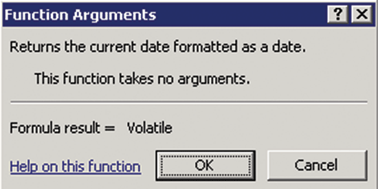
Figure 4

Function argument

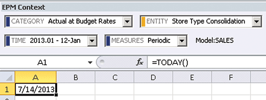
Figure 5

The current date

The second Excel function is used to return the current month. In this function, the MONTH function has been added, and its Serial_number property is set to read the current date in cell A1 (Figure 6).

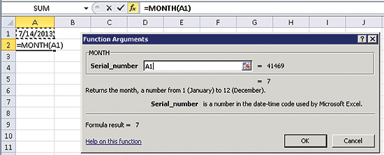
Figure 6

Function argument for the month function

After you click the OK button, the current month is displayed in cell A2 (Figure 7).

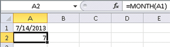
Figure 7

The current month is read from the current date

You use the same technique for the YEAR function to render the current year into cell A3 (Figure 8).

Figure 8

The current year is read from the current date

Next, I show you how to use cell referencing along with the concatenation operator (&) and double quotes(to insert a period) to create the time member in cell E3 (Figure 9). Column E contains the current month.

Figure 9

The year and month are concatenated

You need to change the formula in E3 to insert a 0 if the current month is before 10 (Figure 10). This step is required because the SAP Business Planning and Consolidation time dimension members are in this format (i.e., yyyy.mm). 

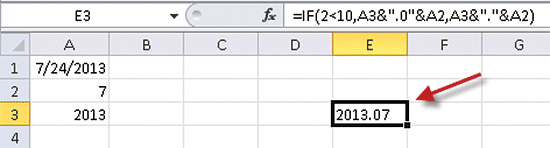
Figure 10

Zero is inserted into the time ID if the current month is before October

Now I explain how to determine prior and future months. First, you determine all 12 months in row 3. To determine the prior three months of your rolling horizon, use the EPMMemberOffset function. Figure 11 shows that you use an Offset of -1 to establish the month in column D.

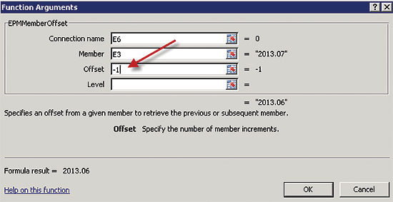
Figure 11

The EPMMemberOffset with an offset of -1

The four parameters of the EPMMemberOffset function are used as follows:

• Connection name: Enter the model ID of the desired connection or leave blank to inherit the current connection
• Member: The starting member, in this case 2013.07 located in E7.
• Offset: The value to decrement or increment from the starting member (the prior month in this case)
• Level: To display the same month last year, for example (I don’t use this parameter in this example).

In Figure 12, you can see that 2013.06 is rendered into D3.

Figure 12

The prior month is rendered into cell D3 via the EPMMemberOffset function

By copying the function in D3 into B3 and C3, you now have the first four months (columns) in place (Figure 13). Row 3 ultimately is hidden from the user because it is only being used to determine the report’s column axis.

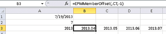
Figure 13

The first four months of your rolling horizon are determined

To determine the eight future months of your rolling horizon, you use the same EPMMemberOffset function, but with an Offset of 1 instead of -1  (Figure 14).

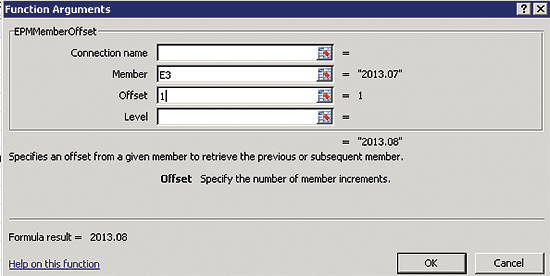
Figure 14

EPMMemberOffset with an offset of 1

Using the EPMMemberOffset for columns F through M provides you with all 12 months for your report (Figure 15).

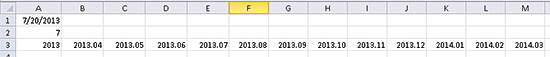
Figure 15

All 12 months have been determined for the rolling forecast

To create a rolling forecast report, you first must have not only time in the column axis but also the category. In addition, because the first three months are always used to display actual data, you can simply type in ACTUAL in B4, C4, and D4 (Figure 16).

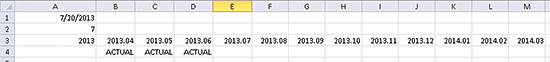
Figure 16

Hard-code the category ID: ACTUAL

Because the current month’s actual data has not been determined yet, it has a forecast category member as do all subsequent months. In my scenario, I want to use a category member of FCST_JUL (i.e., July being the current month), and of course, when August rolls around, it will be FCST_AUG, and so on. Therefore, the category member must be derived from the current year and month.

In the time dimension that I use in my example, there is a Period property that I can use for this purpose. I need to show you this master data from the Web client.  In the Web client, you can access the dimensions via Planning and Consolidation Administration.  Once there, go to Dimensions and select the Time dimension to open up its member sheet (Figure 17). If you look in the Period column in Figure 17 you can see that 2013.01 has a value of JAN, 2013.02 has a value of FEB, and so on.

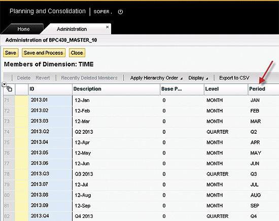
Figure 17

Time dimension members from administration

Now that you have seen the time dimension data, I’ll return to Excel. To derive the category member ID, use the constant text FCST_ and concatenate it with the Period from the current month (Figure 18).

Figure 18

Derive the FCST_

If you look at the function argument for EPMMemberProperty, you can see that the Member parameter has also been locked down via $E$3 so that you can copy it to the months in columns F to M and still retain the reference to E3 (Figure 19).

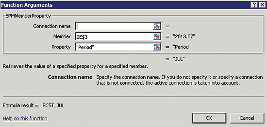
Figure 19

The EPMMemberProperty function

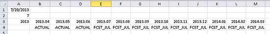
Figure 20

The time and category members are derived

Step 4. Create a New Report with Accounts in the Rows and Time/Category in the Columns

In Figure 21 you can see that I’ve added a report starting in row 7. To add a report, choose Add Report from the EPM ribbon. Drag the account dimension to the rows and time/category into the columns. Because you haven’t yet linked the report’s column axis to the time IDs in row 3 and category in row 4, they display different months, and each column is set to display actual data for every month.

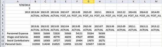
Figure 21

Workbook with the initial EPM report before linking to the derived time and category IDs

Step 5. Change the EPMOlapMember Function to Bring the Current Year, Month, and Category into the EPM Report

In my scenario, the business requirement is to display the current month in column E, the previous three months in columns B-D, and the future eight months in columns F-M so that I have a 12-month rolling horizon. For this scenario I  need to use cell referencing to bring in the desired time ID into the system-generated EPMOlapMember function.

To look at the EPMOlapMember function in cell B7, click the insert function button (fx) in the formula bar (Figure 22). 

Figure 22

EPMOlapMember as generated by the system

The EPMOlapMember function has five parameters. Only the first parameter is available for cell referencing; the system controls the rest. Therefore, you need to reference the current year/month into the first parameter of this function. You do this by accessing the formula in the function bar, add B3 for example in the first parameter following by a comma. Then delete one of the unused parameters.

In Figure 23, you can see that time ID in B7 is now referenced into the EPMOlapMember function.

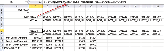
Figure 23

The current year.month is referenced into the EPMOlapMember function in B7

By copying B7 to columns C through M, the EPM report now has the 12 months that you need (Figure 24).

Figure 24

The EPM Report with time determined

By using the same technique of referencing the EPMOlapMember function to the category IDs in row 4, you also derive the category member in the EPM report in row 8 (Figure 25).

Figure 25

EPM report with the column axis complete

Because my business scenario is to only allow data entry for the forecast months, I need to add a property to the category dimension. This property then is used in the formatting sheet to prevent data entry for actual months and allow data entry for the forecast months.

Step 6. Set Up a Category Dimension Property to Be Used for the Formatting

To add a property to a dimension, you need to first access the Web client (Figure 26).

Figure 26

Web client

Now click Planning and Consolidation and then click the Administration tab. Click Dimensions and then select Category (Figure 27). 

Figure 27

How to access the Category dimension in Administration

Click the Edit Structure button, and in the Structure of Dimension: CATEGORY, choose Add. Enter a property ID and Name such as LOCK with Number of Characters of 1 (Figure 28).

Figure 28

Category dimension with LOCK property

After clicking the Save button, choose Members of Dimension: CATEGORY. Enter in a value of Y for Actual and N for the category members for the Jan-Dec forecasts (Figure 29).

Figure 29

Category members with LOCK property values

Now you can go back to Excel and set up the formatting.

Step 8. Format Actual Months to Be Locked for Data Input and Forecast Months to Data Input

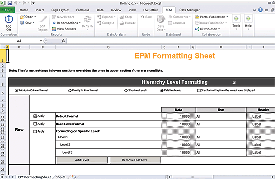
Figure 30

The initial EPMFormattingSheet

Scroll down to the Dimension Member/Property Formatting section and activate it by checking the box in cell J52 (Figure 31).

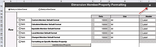
Figure 31

Activate Dimension Member/Property Formatting

Because category is in the columns, you scroll down to the Column formatting section and check the Apply checkbox in C99 to activate Formatting on Specific Member/Property (Figure 32). 

Figure 32

Activate Formatting on Specific Member/Property

To select a member property, click the Add Member/Property button. The EPM formatting sheet for member/property appears (Figure 33).

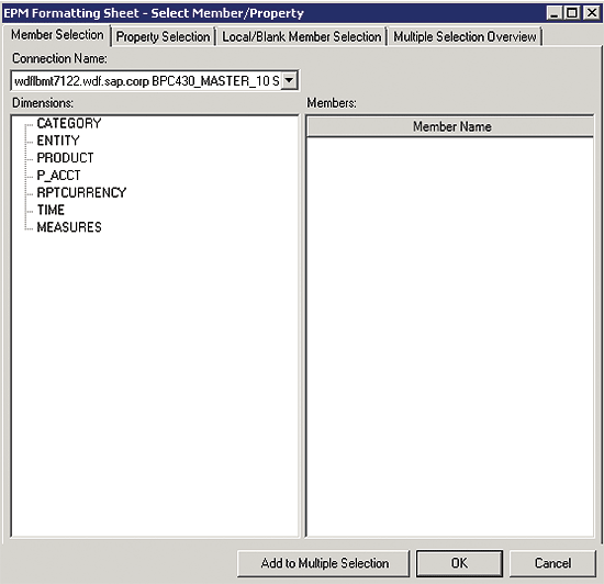
Figure 33

The dialog to add a member property

Because you need to control data entry for the LOCK category member property, go to the Property Selection tab, select the CATEGORY  Dimension, the LOCK Property, the = Operator, and a Value of Y (Figure 34). (This is for the Actual member ID).

Figure 34

Select the LOCK property value = Y

To adopt the select, click OK and then you can see the results in cell D95 (CATEGORY.LOCK = Y) in the screen shown in Figure 35.

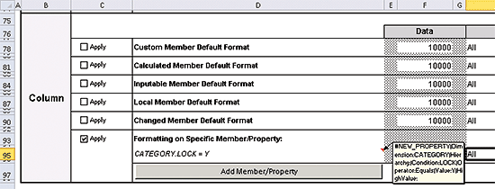
Figure 35

Member property setting for actual months

Using the same technique, you can see a similar setting for the LOCK property value of N, which is used for forecast months (Figure 36).

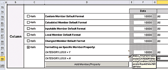
Figure 36

Member property setting for forecast months

Now you need to format the Data and Label values. The actual cells have a gray pattern. Therefore, the pattern in cell F95 is set to gray. The forecast cells have a light blue pattern. Therefore, the pattern in cell F98 is set to light blue (Figure 37).

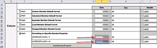
Figure 37

Formatted data cells

In addition, the user should receive an error when attempting to input actual data. To set this up,  right-click cell F95 and select EPM > Lock Selected Cells (Figure 38).

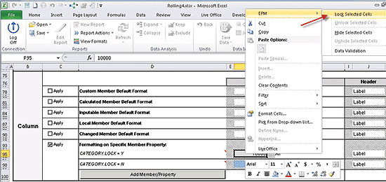
Figure 38

Lock selected cells

To close the EPMFormattingSheet, choose View Formats. To render the new formatting, choose Refresh.  Now you can see the results in Figure 39. Actual months are in gray, whereas the forecast months are in light blue by design.

Figure 39

Initial results of member property formatting

Just to make sure everything is working, hard-code in a date in A1 for August 20, 2013. You can see in Figure 40 that each month has been advanced by one, and that the forecast category is now FCST_AUG. 

Figure 40

Test for a date in the next month

Before proceeding with the data input testing, you need to do a little housekeeping. First,  get rid of the green indicators (they signify unprotected formulas) in the column and row axis cells. In File > Options > Formulas, deselect Enable background error checking (Figure 41).

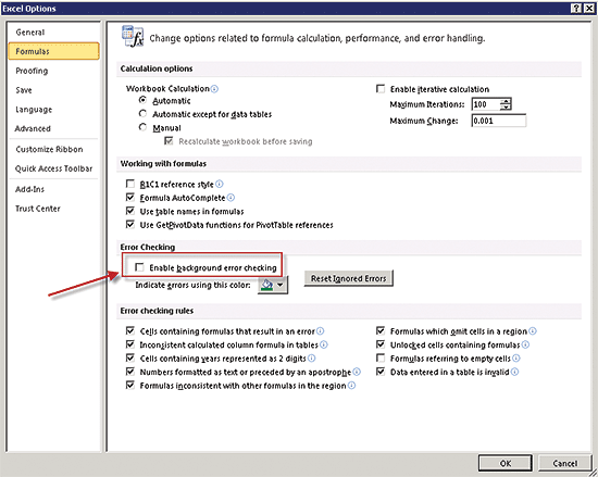
Figure 41

Turn off background error checking

Now you can see in Figure 42 that there are no longer any unprotected formula errors.

Figure 42

Report output with no unprotected formula errors

Next, hide rows 1-4 by grouping them. Proceed by highlighting rows 1-4 and then choose Data > Group > Group… (Figure 43).

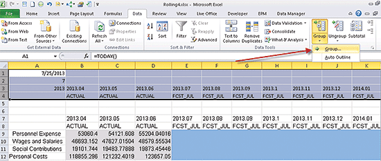
Figure 43

Turn on grouping for rows 1-4

Note that in Figure 44 the rows 1-4 are now hidden and a button (with a + symbol) is available to open them back up during construction of the input form.

Figure 44

Rows 1-4 hidden in a group

Next, turn off the Gridlines and Headings. Go to View and  deselect the boxes for Gridlines and Headings (Figure 45).

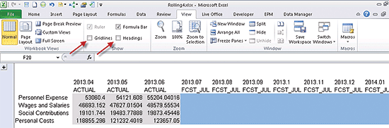
Figure 45

Turn off Gridlines and Headings

Next, put a border around the data cells, and right justify the column labels. Select View Formats to open the EPMFormattingSheet. In Figure 46, note that  F95 and F98 now have a border. You also need to set the data cells to numeric with a comma separate and no decimals. Also, cells J95 and J98 are now right justified. 

Figure 46

Format a border on the data cells and right justify the column labels

To render the new formats, click View Formats. Go to sheet 1 and click Refresh. You can see in Figure 47 that you now have a nicer looking report. 

Figure 47

Report with borders on data cells and column labels right justified

Now you can proceed with the final test to make sure no one can input actual data. Because the formatting is already in place (actuals are set to Lock Selected Cells), you just need to protect the workbook. Go to Tools > Options > Sheet Options. In the Protection tab select Protect Workbook and enter a password (Figure 48).

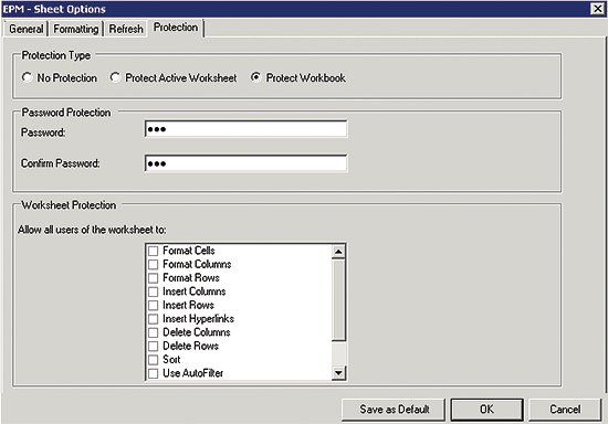
Figure 48

Protect the workbook

After closing the EPM-Sheet Options dialog and entering a value for the first actual month, you can see in Figure 49 that an error message appears. You can also see that View Formats is grayed out. This prevents anyone from going into the EPMFormattingSheet and turning off Lock Selected Cells.

Figure 49

An error when trying to enter in a value for actuals

Now that you’ve proven that no one can enter actual values, enter and save a value for a forecast month such as August in this case. In Figure 50 you can see that the value of 57,000 has successfully been entered and saved.

Figure 50

Success when entering and saving a forecast value

You now know how to create a rolling forecast input form.

Charles "Tim" Soper

Charles “Tim” Soper is a senior education consultant at SAP. For the last 17 years, he has been teaching SAP classes on a variety of topics in financial and managerial accounting, business warehouse, business consolidations, and planning. He is the planning and consolidation curriculum architect and has written SAP course manuals. He also works as an SAP Senior Educational Consultant. Early in his career, he worked for Eastman Kodak Company in Rochester, NY, as a senior financial analyst. He has an undergraduate degree in economics and an MBA in finance from the University of Rochester.

You may contact the author at Charles.Soper@sap.com.

If you have comments about this article or publication, or would like to submit an article idea, please contact the editor.