Learn how to increase the accuracy of the current forecast models in SAP materials management (MM). This alternative strategy consists of combining different forecasting models by placing weights on individual forecasts. The idea behind the combination of forecasting techniques is that no forecasting method is fully appropriate for all situations. You can apply this improved forecasting solution to any kind of business using standard SAP tools to take forecasting to the next level.
Key Concept
Trends can be either deterministic or stochastic. When attempting to forecast a trend, the deterministic component defines an exact relationship between variables. Its counterpart is the stochastic component, which is a collection of random variables and often represents random values over time.
SAP materials management (MM) provides the following forecast models: Constant, Moving Average, Weighted Moving Average, Trend, Seasonal, and Seasonal Trend. Through experience, we know that one model doesn’t always completely fit or address a forecasting situation. We have found that by combining different models, the new forecast is more accurate and improves the decision-making process.
To determine when future purchases need to be made, a company can use a Combined Forecast Model (CFM) approach, which is an enhancement of the standard forecast methods available in the MM module. CFM can be triggered by using program RMPR1001. You only need the MM module and its inventory management (IM) submodule implemented. Of course a company would usually have at least the financial accounting (FI) and sales and distribution (SD) modules in place as well.
We explain the underlying mathematical analysis of SAP forecasting models and the process of combining forecasts and giving weight to the results. After covering how to evaluate forecast accuracy, we walk you through the process of choosing a forecast model and then executing it, which includes preparing your master data. Next, we show you how to import forecast values. This step includes displaying the forecast values in the material master and listing the stock requirements. Finally, we show you how to execute the MRP run.
To illustrate our point, we analyze the accuracy of a forecast scenario over a 12-month period using a combined and weighted forecast process. For basic information about forecasting, see the quick tip “Understanding SAP Forecasting Models.”
Combining Forecast Models
The forecasting performance of a given model is time-varying. This means that the selection of an optimal forecasting model among many competitors (where optimality is measured with some statistical criteria) depends on the information set, model specification, and sample period. Combining methods can compensate for the weakness of each forecasting model under particular conditions because it accounts for the time-varying forecasting ability of alternative models.
Note
Although there is broad consensus that appropriate combinations of individual forecasts often improve forecast accuracy, the literature has not yet converged on a particular set of forecast weights to be implemented when constructing combined time series. Evidence indicates that combining forecasts through a simple equal weight (EW) scheme produces more accurate forecasts. We propose a simple combination procedure that places a constant equal weight to each model at each time period, with the weight equal to 1/k (where k is the number of alternative models used in forecasting). Several studies have shown that the equal-weighted combination forecast is quite successful when compared with other weighting procedures.
Evaluating Forecast Accuracy
Our experiment consisted of forecasting six alternative models and the evaluating their relative forecast performance in terms of accuracy. The models we used were a constant-no-change random walk, a constant model, a trend and season model, a trend model, a seasonal model, and a combining forecast model with EWs. To evaluate their accuracy, we used two standard measures: mean absolute error (MAE) and root-mean-squared prediction error (RMSPE). In particular, we computed the MAE and the RMSPE to measure how close the forecasts were to the actual historical data using the formula shown in Figure 1.
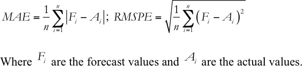
Figure 1
Formula to measure accuracy of the forecasts
Table 1 shows the relative MAE and RMSPE with respect to the EW model for each competing model. A number lower than one means that combining individual models with equal weight leads to lower forecast errors and higher forecast accuracy. The results show that the equal weight is the top-performing model according to both measures of forecast accuracy.
Table 1
Comparing forecast accuracy
The last column of the table also reports the improvement obtained (in percentage) when using the EW model rather than each individual model. For example, using EW instead of the random walk model produces an improvement in accuracy equal to more than 6%, according to the RMSPE indicator of performance. We conclude that combining forecasts with EW would improve the decision-making process for the future material consumption.
To use this CFM in an SAP system, we uploaded the forecasting values to a standard SAP program. The details of this program and the steps needed to adopt the forecasting values are covered in the “Import Forecasts Values” section. However, we want to provide a brief introduction to the planning method, referred to as Consumption-Based Planning (CBP) in MM, and explain the important details that influence forecast accuracy of the material master data.
Choosing and Executing the Forecast Model in SAP MM
It is critical to choose and execute the forecast model or models in SAP MM that are the most relevant for the forecast-based planning procedure. To begin you need to prepare the master data and then you create the material requirements planning (MRP) views.
Master Data Preparation
You can choose the appropriate forecast model for material/plant combination, creating the forecasting view in the material master using the transaction MM01 or by following menu path SAP Menu > Logistics > Material Management > Material Master > Material > Create (general) > Immediately. After you enter the material code (2) and plant (0004) and select the Forecasting view, the system displays the screen shown in Figure 2.
Figure 2
Forecasting view
Note that in our example, as shown in Figure 2, we have selected the option N as the forecast model to be defined using an external model (to enhance the standard models available in the system).
Table 2 provides the description of the fields required to define the appropriate forecast model based on your needs.
Table 2
Explanation of SAP parameters relevant for defining forecast models
After entering the appropriate values, you specify the consumption values. Note that the system automatically updates those values based on the posting done in the IM module. Figure 3 shows the consumption values specified or updated.
Figure 3
Consumption values
Tip!
Set up the forecasting profile to store defaults independently of a material master record and facilitate data entry and data management. Define the following values:
- Fields that are filled with values when forecast data is entered in the material master record
- Values allowed in these fields
- Values that can be overwritten and those that cannot
To create a forecast profile, use the customizing transaction MP80 or follow menu path SAP Menu > Logistics > Materials Management > Material Master > Profile > Forecast Profile > Create.
To ensure that the new forecasted method is used during the planning of the material, you need to maintain the value VV as MRP Type in the MRP-1 view (Figure 4).
Figure 4
MRP 1 view
MRP Views
To use the basic SAP-provided planning tools, you need to create three MRP views for material/plant combination. To create the MRP views, use transaction MM01 or follow menu path SAP Menu > Logistics > Material Management > Material Master > Material > Create (general) > Immediately. Enter the material code, select a plant, and specify the MRP procedure settings for the first MRP view, as shown in Figure 4.
Next, specify the appropriate settings in the MRP 2 view (in particular the external procurement type indicator as F and the safety stock details). In the MRP 3 view among the planning parameters you can specify the period indicator for forecasting calculation and the availability check details, as shown in Figures 5 and 6.
Figure 5
MRP 2 view
Figure 6
MRP 3 view
At this stage, you have completely maintained the basic master data.
Import Forecast Values
Forecast values are generally calculated by the system as part of the forecasting process and then updated in the material master record. However, you can manually enter forecast values that form the basis of the planning run, or import them from a legacy system or external system. To import forecast values from a legacy system or another external system into the material master, follow these steps:
Step 1. To run the standard program RMPR1001, execute transaction SE38 (usually it is scheduled in background). You can use the program RMPR1001 to transfer forecast values from external systems to the SAP system. Exits are available for program RMPR1001 to fulfill specific business requirements.
Note
Before running program RMPR1001, you must specify in the forecast view of the material master the method as value N – No forecast/external model (Figure 2).
Figure 7 shows two options for the method to adopt an external forecast. I’m using the option T to test the forecast results, but you should use option U.
Figure 7
Selection options
Figure 8 shows the details of the selection of this report. The indicator M specifies the period in which the material’s consumption values and forecast values are managed. In this case it is in a monthly time bucket.
Figure 8
Selection screen of the report RMPR1001
Step 2. Press the Enter key and the system provides the details listed, as shown in Figure 9.
Figure 9
Forecast values obtained from the CFM
Step 3. Click the Adopt button so the system can confirm the transfer of the forecast values, as shown in Figure 10.
Figure 10
Confirmation of the forecasts transfer
Step 4. Press the Enter key. Figure 11 shows the details of forecasts adopted from an external source.

Figure 11
Forecast values adopted from the external Excel file
Tip!
You can use program RMPR1001 to transfer forecast values from external systems to an SAP system.
The program works as follows:
- 1. The program searches for the material/plant combination defined for the external forecast.
- 2. Using user exit EXIT_SAPLMPR1_002, you set a filter on the materials to be forecast externally.
- 3. The program calls user exit EXIT_SAPLMPR1_001 and transfers information on the materials to be forecast.
- 4. The user exit must have the forecast values from the external system at its disposal. You can do this by creating a new enhancement project using transaction CMOD. The business department would provide input to the developer. This process is transparent to end users.
- 5. After the user exit is run, the forecast values are posted in the SAP system.
Display the Forecast Value in the Material Master
To view the forecast values in the material master, use transaction MM03 or follow menu path SAP Menu > Logistics > Material Management > Material Master > Material > Display. Enter the material code, select the plant, and specify the forecasting view (Figure 12).
Figure 12
Forecast values adopted from the external source (i.e., an Excel file)
If you want, you can display the forecast results using the graphic icon  (shown in Figure 12).
The graphics are shown in Figures 13 and 14. In Figure 13, in a monthly bucket you can see the original forecasts generated based on the historical consumption values.
Figure 13
Forecasting results (interactive graphics)
Figure 14
Forecasting adjusted results (graphical display)
In Figure 14, you can see the simulation of the adjusted forecast and consumption results in a monthly bucket. Note the following details:
- In yellow, the details of the historical corrected consumption values
- In blue, the details of the historical originating consumption values
- In red, the originating forecasting values
- In green, the corrected forecasting values
Note
In MM, you can execute a forecast calculation for the standard SAP methods in the following ways:
- At a single material and plant level, use transaction MP30 or follow menu path SAP Menu > Logistics > Material Management > Material Requirements Planning (MRP) > Forecast > Individual forecast > Execute.
- At the total materials and plant level, use transaction MP38 or follow menu path SAP Menu > Logistics > Material Management > Material Requirements Planning (MRP) > Forecast > Total forecast > Execute.
- At a single material and plant level, use transaction MM02 or follow menu path SAP Menu > Logistics > Material Management > Material Master > Material > Change.
Stock Requirement List
To check the results of the forecast run, use transaction MD04 or follow menu path Logistics > Materials Management > Material Requirements Planning (MRP) > MRP > Evaluation > Stock/Reqmts List (Figure 15).
Figure 15
Forecasting results visible in the stock requirement list
The MRP element ForReq represents the forecast requirements, which were calculated based on the forecast model selected and other forecast parameters defined in the forecasting view of the material master.
Stock Requirement List
To react to the demand created by the forecasts, run the MRP. This is usually done via a background job, but in our example, we used transaction MD03, which you can execute by following menu path Logistics > Materials Management > Material Requirements Planning (MRP) > MRP > Planning > Single-Item, Single-Level (Figure 16).

Figure 16
Parameters for the MRP run
Results of the MRP Run
To check the results of the MRP run, use transaction MD04 or follow menu path Logistics > Materials Management > Material Requirements Planning (MRP) > MRP > Evaluation > Stock/Reqmts List (Figure 17).
Figure 17
Results of the MRP run
At this point in the process, the system has also created the purchasing requisitions (in the opening period, which in this case is 10 working days) and the planned orders outside the opening period.

Gaetano Altavilla
Dr. Gaetano Altavilla is a senior SAP practice manager. His focus is on pre-sales, delivery of SAP application solutions for large international corporations, and SAP knowledge management in Europe, the Middle East, and Africa (EMEA).
In his 18 years of SAP application experience working for many multinational companies, such as Procter & Gamble and Hewlett-Packard, he has covered a wide range of ERP logistic areas, focusing on the MM, WM, SD, LES, PP, PP-PI, PLM (QM, PM, PS) modules, as welll as CRM (TFM), SRM (EBP), SCM (SAP APO), and MES (ME) components.
Dr. Altavilla holds a degree with first-class honors in mathematics from the University of Naples and is certified in many SAP modules: SAP Logistics Bootcamp, SAP MM, SD, LE (SHP/WM/LE), PP, PLM (PM, QM, PS), SRM, CRM, SCM (APO), SCM (TM), FI, CO, and Solution Manager. He also has experience in ABAP/4 and application link enabling (ALE) and IDocs. He has participated in numerous industry conferences, such as the SAP Skills Conference in Walldorf at SAP SE.
You may contact the author at Gaetano_altavilla@hotmail.com.
If you have comments about this article or publication, or would like to submit an article idea, please contact the editor.

Prof. Carlo Altavilla
Prof. Carlo Altavilla is associate professor of economic policy at the University of Naples “Parthenope,” Italy, where he teaches microeconomics and econometrics. Prof. Altavilla completed his undergraduate studies at the University of Naples “Federico II” in Italy, received a master’s degree in economics and finance, and completed a PhD in economics at the Catholic University of Leuven (Belgium). Upon completing his PhD, he was appointed assistant professor and then associate professor of economics at the University of Naples “Parthenope.” He has been a visiting scholar at Columbia University (New York, USA) and consultant for several national and international institutions, including the European Central Bank. His research interests focus on applied econometrics and time-series analysis. He has published in a wide range of international journals including the Journal of Money Credit and Banking, Applied Economics, International Journal of Finance and Economics, and Journal of Economic Behavior and Organization. You may contact Prof.
You may contact the author at altavilla@uniparthenope.it.
If you have comments about this article or publication, or would like to submit an article idea, please contact the editor.