Management profitability analysis reporting requires allocation of financial data such as supply and delivery freight costs at a detailed customer and product level, compared to a much higher level such as company code and strategic business unit (SBU). Management profitability analysis is similar to profitability analysis (CO-PA). It is a BI-based solution that provides complete customer and product level profitability analysis via allocation of financial data (i.e., expenses) that lives outside of the sales and distribution (SD) module. This reporting requires that the higher level financial data be allocated down to a customer and product level based on percentages of quantity or volume by the customer and product sales and distribution data.

The business runs a suite of reports and management dashboards on this allocated data with visibility at all levels of the organization (from the company level to product lines to individual customers and products) facilitating the ability to make better decisions related to customer pricing and product mix. The model provides a consistent profit distribution to allow comparison across regions, strategic business units, and product lines with the ability to drill down to sales orders, deliveries, and billing documents.

At my company we developed several allocation processes with complex functionality using the custom approach described in this article, as the standard functionality didn’t meet the requirements. I selected the simplest of all those allocation processes we developed and explain it in detail. 

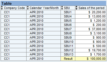
Let’s take a quick look at the financial, configuration, and SD data that needs to be read for this process. Figure 1 shows the financial data, which is at a company code level for Calendar Year/Month APR 2010. You need to allocate the Sales of the period amount; in my example, $100,000.00.

Figure 1

Financial data to be allocated

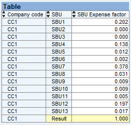
Figure 2 shows the configuration data. It lists all the SBUs for company code CC1 and the corresponding percentages.

Figure 2

Configuration data

Figure 3 shows the SD data that is at a detailed level, such as Company code, Customer number, Material number, Sales document, Billing document, Delivery, SBU, and Sales Volume (MT) for calendar year/month APR 2010 (the data in the figure is filtered on the calendar year/month for which the allocation is being run; in this example it is APR 2010). The amount of $100,000.00 from finance for company code CC1 will be allocated at this detailed level based on the percentage of the sales volume.

Figure 3

SD data

Overview of the Process

Step 1. Each finance data record generates multiple records based on the number of SBUs defined in the configuration data for that company code. All of these newly generated records have the same characteristic values as the original record except that SBU is populated on each one of them. The sales of the period key figure values are based on the percentages of the corresponding SBU. I refer to this process as a high-level allocation process in the rest of this article. The data that is generated in this process is stored in a high-level InfoCube.

Figure 4 shows how the finance record at the company code level (with a Sales of the period amount of $100,000.00) generated multiple records at the company code and SBU levels based on the SBUs and their corresponding percentages from the configuration data. The $100,000.00 amount was split between SBUs based on the percentages in the configuration data.

Figure 4

Multiple records generated

Step 2. Generate a percentage calculation based on the sales volume at the company code, calendar year/month, customer, and material levels for each detailed SD record that is at the document level (e.g., sales, billing, and delivery).

• Get the summarized sales volume of SD data at the company code, customer, and material levels for the calendar year/month for which the allocations are being done
• For each detailed SD record at the document level (e.g., sales, billing, and delivery), get the summarized sales volume calculated in the previous step for the corresponding company code, customer, and material levels, and calculate the percentages for the detailed records — for example, the sales volume for the detailed record divided by the summarized sales volume for the corresponding company code, customer, and material levels.

Step 3. For each detailed record in SD that has the sales volume percentage calculated in the previous step, find the matching record at the high level (step 1 above) using the company code and SBU as matching criteria. Get the dollar amount from the high level and use the percentage that was calculated in step 2 above for that SD record to get the final allocation dollar amount for that record. The process that performs steps 2 and 3 is referred to as the low-level allocation process in the rest of this article. This generated low-level allocation data is stored in the low-level allocation InfoCube.

List of Required Objects

Following is a list of all the objects that you need to create in SAP NetWeaver BW, Integrated Planning (IP), Business Planning and Simulation, and ABAP, plus the role of each object in the allocation process.

SAP NetWeaver BW:

• The extraction cube storing the finance data that needs to be allocated. The corresponding data transfer process object and transformation object are required for data load to the extraction cube from the finance cube.
• The configuration cube storing configuration data (i.e., a list of SBUs for each company code and the percentage that needs to be allocated to each SBU). This data is maintained using integrated planning.
• The high-level cube storing the generated finance data at the company code and SBU levels using the high-level allocation process
• The low-level cube storing the generated allocation data by the low-level allocation process
• The sales cube storing detailed SD data and the corresponding data transfer process object and transformation object required for data load to the sales cube from SD

Integrated Planning:

• The integrated planning objects, such as aggregation level, input ready query, and workbook on the aggregation level for adding and maintaining the configuration data

Business Planning and Simulation:

• The planning area (PA1) for the extraction cube that has finance data at a company code level
• The planning area (PA2) for the high-level cube for which data is generated by the high-level allocation process, which has finance data at a company code and SBU levels
• The multi-planning area (MPA1) on the above two planning areas
• The planning function of type Exit on the multi-planning area (MPA1) calling a function module that has the logic for the high-level allocation process
• The planning sequence to run the planning functions in the background
• The planning area (PA2) for the high-level cube that has finance data at the company code and SBU levels. This is the same planning area as in step 2.
• The planning area (PA3) for the low-level cube for which data is generated by the low-level allocation process, which will have the detailed allocation data
• The multi-planning area (MPA2) on the above two planning areas
• The planning function of the type Exit on the multi-planning area (MPA2) calling a function module that has the logic for the low-level allocation process
• The planning sequence to run the planning functions in the background

ABAP:

• The function module that has logic for the high-level allocation process (i.e., to read the finance data from the extraction cube which is at the company code level, generate the data at the company code and SBU levels based on the configuration cube data, and store the generated data in the high-level cube)

• The function module that has logic for the low-level allocation process (i.e., to calculate the percentage based on sales volume at the company code, calendar year/month, customer, and material levels for each detailed SD record that is at the document level (sales, billing, and delivery) and to calculate the final allocation dollar amount for that detailed SD record by looking up the corresponding high-level data record.

Planning Objects

Following are step-by-step instructions for creating some key planning objects. In transaction BPS0 select Planning > Planning area > Create. Provide the technical name of the planning area and the description and click the Create button (Figure 5).

Figure 5

Create the planning area

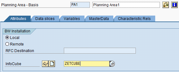
Provide the technical name of the real time InfoCube on which this planning area is based (Figure 6). Click the save icon.

Figure 6

Planning area details

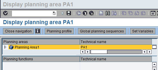
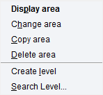
Once the planning area is created, select the planning area (Figure 7), right-click, and select Create level (Figure 8) which shows a new screen (Figure 9). Provide the technical name of the planning level and description and click the Create button.

Figure 7

Display the planning area

Figure 8

Planning area selections options

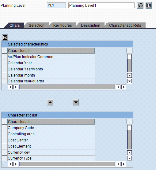
Figure 9

Create the Planning Level

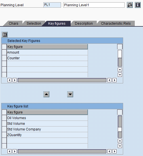
Select the characteristics (Chars) (Figure 10) and Key figures (Figure 11) into the level from the list of all the characteristics and key figures from the underlying InfoCube. Provide selection criteria if any. For example, if the allocation is done for APR 2010, then either enter 04/2010 in the Calendar month field after clicking the Selection tab or use a variable.

Figure 10

Select the characteristics into the level at which the allocation needs to be performed

Figure 11

Select the required key figure and then provide the selection criteria

Select the save all icon (Figure 12).

Figure 12

Save the planning level

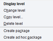
Once the planning level is created, select the level (Figure 13), right-click, and select Create package (Figure 14). Then provide the technical name of the package and a description (Figure 15).

Figure 13

Select the planning level

Figure 14

Planning level selection options

Figure 15

Create a planning package

Select the save all icon (Figure 16).

Figure 16

Save the package

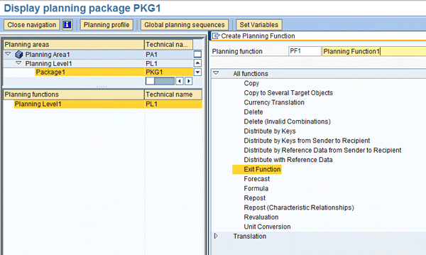
Once the package is created, click Package1 under Planning Level1 and right-click the Planning level displayed under the Planning functions section (Figure 17). Then select Create Planning Function.

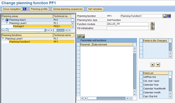
From the list of available functions, select Exit Function (Figure 17) which takes you to the next screen (Figure 18). Provide the Function module name, which has the allocation business logic. From the list of fields from the Planning level, select the fields whose values will be changed during the allocation process and move them to the Fields to Be Changed section (Figure 18). Click the save all icon.

Figure 17

Select Exit Function

Figure 18

Select the function module

The following section gives overviews of the business logic in the ABAP function modules (high level and low level), the framework used by the allocation processes, and of the structure and importance of hashed table XTH_DATA.

High- and Low-Level Allocation Business Logic

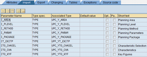
In transaction SE37 provide the function module name that was specified in the planning function of type Exit (Figure 18) and select display. Figures 19 and 20 show the Import and Changing parameters of the function module. You use two function modules, one for the high-level allocation (Multi Planning area MPA1 > Planning level > Planning function) and one for the low-level allocation (Multi Planning area MPA2 > Planning level > Planning function).

Figure 19

Function module Import parameter details

Figure 20

Function module Changing parameter details

High-Level Allocation Process

Steps 1, 2, and 3 below explain the source codes of the function module that has logic for the high-level allocation process. This process reads the finance data from the extraction cube which is at the company code level and then generates the data at a lower level (i.e., the company code and SBU levels), based on the configuration cube data. The generated data is then stored in the high-level cube. The importance of hashed table XTH_DATA, its structure (characteristics and key figures), and some of its special characteristics are also covered.

Step 1. Create an internal table (int_config_data) to store the configuration data read from the configuration cube and create a corresponding work area (wa_config_data).

Step 2. Read the data from the configuration cube to the internal table:

• Create the following data objects that store the names of the characteristics and the key figures that need to be read from the configuration cube, and to set the filter criteria if any.

DATA:   g_s_sfc    TYPE rsdri_s_sfc (Delivered Structure),

        g_t_sfc    TYPE rsdri_t_sfc (Delivered Table of Line Type rsdri_s_sfc),
        g_s_sfk    TYPE rsdri_s_sfk (Delivered Structure),
        g_t_sfk    TYPE rsdri_t_sfk (Delivered Table of Line Type rsdri_s_sfk),
        g_s_range  TYPE rsdri_s_range (Delivered Structure)

        g_t_range  TYPE rsdri_t_range (Delivered Table of Line Type rsdri_s_range).

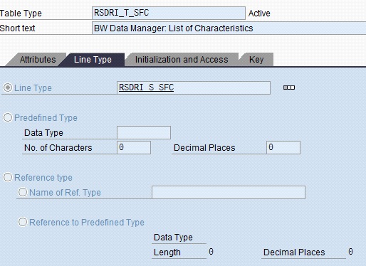
Figures 21 and 22 show one of the above-delivered structures and table types.

Figure 21

Delivered structure

Figure 22

Table type

• Use this code in the function module (used for high-level allocation) to set the characteristics and key figures that need to be read from the configuration cube and set the filter criteria if any.

  CLEAR g_s_sfc.
  g_s_sfc-chanm    = 'OSBU'.
  g_s_sfc-chaalias = 'OSBU'.                           INSERT g_s_sfc INTO TABLE g_t_sfc.

  CLEAR g_s_sfc.
  g_s_sfc-chanm    = '0COMP_CODE'.
  g_s_sfc-chaalias = '0COMP_CODE'.

  INSERT g_s_sfc INTO TABLE g_t_sfc.

  CLEAR g_t_sfk.
  CLEAR g_s_sfk.
  g_s_sfk-kyfnm    = 'OSBUPERC'.
  g_s_sfk-kyfalias = 'OSBUPERC'.

  INSERT g_s_sfk INTO TABLE g_t_sfk.

  g_s_range-chanm    = 'OEXPTYPE'.
  g_s_range-sign     = 'IN'.
  g_s_range-compop   = 'EQ'.
  g_s_range-low      = 'FRT'.
  APPEND g_s_range TO lt_range.

  RSDRI_TH_SFC = g_t_sfc[].
  RSDRI_TH_SFK = g_t_sfk[].

• Call function module RSDRI_INFOPROV_READ and pass the objects that were created in the previous step. This reads the data from the configuration cube and stores it in the internal table.

CALL FUNCTION 'RSDRI_INFOPROV_READ'
         EXPORTING
           I_INFOPROV            = ‘Configuration cube'
           I_TH_SFC              = RSDRI_TH_SFC – List of Characteristics that needs to be read
           I_TH_SFK              = RSDRI_TH_SFK  – List of Key figures that needs to be read
           I_T_RANGE             = LT_RANGE – Filter criteria
*          I_AUTHORITY_CHECK     = L_AUTHORITY_CHECK
                           I_USE_AGGREGATES      = ‘ ‘
           I_ROLLUP_ONLY         = ' '
           I_CURRENCY_CONVERSION = ' '
           I_PACKAGESIZE         = -1
         IMPORTING
           E_T_DATA              = ‘int_config_data’ – Internal table where the data is stored

         CHANGING
           C_FIRST_CALL          = L_FIRST_CALL
         EXCEPTIONS
           NO_AUTHORIZATION      = 3
           TRANS_NO_WRITE_MODE   = 4.

This internal table will be used for further processing in the function module.

Step 3. This section explains the structure and importance of hashed table XTH_DATA and how the records in it are processed. As mentioned in the earlier sections, this function module for high-level allocation is called from Multi Planning area MPA1 > Planning level > Planning function. This multi-planning area MPA1 is created on planning area (PA1) for the extraction cube. The extraction cube has finance data at the company code level and planning area (PA2) for the high-level cube. Data was generated for it by the high-level allocation process, which has finance data at the company code and SBU levels.

XTH_DATA is available in the function module and has data from the multi-planning area MPA1.

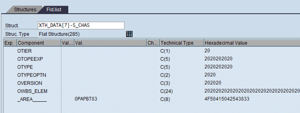
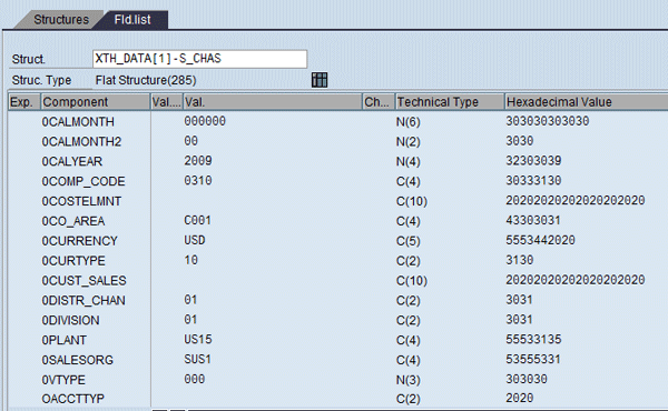
Figure 23 shows the structure of XTH_DATA (debug mode). It has structure S_CHAS, which has all the characteristics and values (Figures 24 and 25), and structure S_KYFS, which has all the key figures and values (Figure 26) for each record. These records come from both the extraction cube and the high-level cube. However, in this scenario there is no data in the high-level cube as the allocation for that closing month is not yet run. Therefore the high-level allocation data is not yet generated.

Figure 23

Structure of hashed table XTH_DATA

Figure 24

Field list (characteristics) in hashed table XTH_DATA

Figure 25

Field list (characteristics) in hashed table XTH_DATA

Figure 26

Additional field list (key figures) in hashed table XTH_DATA

Create FIELD-SYMBOLS <fs_xth_data> to hold a single record of XTH_DATA and create FIELD-SYMBOLS for each of the characteristics and key figures of the underlying cubes. Create FIELD-SYMBOLS only for those characteristics and key figures that will be used in the selection criteria later or whose values will be changed.

Example:

    FIELD-SYMBOLS:  <fs_xth_data> TYPE ANY,

                <fs_xth_data_sbu> TYPE ANY,

                <OSBU> TYPE ANY,
                <ZCOMP_COD> TYPE ANY,
                <0CALMONTH> TYPE ANY,
                <0CO_AREA> TYPE ANY,
                <0SALES> TYPE ANY,

                <XPLNAREA> TYPE ANY,

                <XPLNAREA_1> TYPE ANY,

                <0SALES_1> TYPE ANY.

Process records in XTH_DATA by looping through each record. The records in XTH_DATA are the financial data from the extraction cube. See the loop statement below.

     LOOP AT xth_data assigning <fs_xth_data>.

As mentioned earlier there are two structures in XTH_DATA. The characteristics for each record can be retrieved from the structure S_CHAS and the key figures can be retrieved from the structure S_KYFS. See the assign statement below, which reads ZCOMP_COD and _AREA_____ characteristics from the structure S_CHAS and the 0SALES key figures from structure S_KYFS.

The _AREA_____ Characteristic in the structure S_CHAS is a special characteristic that is used to identify the source of the record whether the record is from the extraction or high-level cube. The IF condition below looks for this characteristic value and then the processing is done only if the record is from the extraction cube (finance data) but not from the high-level cube.

ASSIGN COMPONENT 'S_CHAS-_AREA_____' OF STRUCTURE <fs_xth_data>
                   TO <XPLNAREA>.
IF <XPLNAREA> EQ 'planning area associated with high level cube'.
    continue.
endif.

ASSIGN COMPONENT 'S_CHAS-ZCOMP_COD' OF STRUCTURE <fs_xth_data>
              TO <ZCOMP_COD>.

ASSIGN COMPONENT 'S_KYFS-0SALES' OF STRUCTURE <fs_xth_data>
              TO <0SALES>.

Create another FIELD-SYMBOL <fs_xth_data_sbu> and copy data from <fs_xth_data> to <fs_xth_data_sbu>. See the assign and move-corresponding statements below.

assign lr_wa->* to <fs_xth_data_sbu>.
MOVE-CORRESPONDING <fs_xth_data> TO <fs_xth_data_sbu>.

This <fs_xth_data_sbu> has the same data as <fs_xth_data> (the original data from the extraction cube — i.e., finance data). You set the SBU, the planning area characteristics, and the sales key figure by reading the configuration data from the internal table for the corresponding company code.

Read the configuration data for each record of XTH_DATA. Note that <ZCOMP_COD> used in the loop statement below is the company code from the extraction data record from XTH_DATA. This returns a list of all SBUs for that company code and the percentage split for each SBU.

LOOP AT int_config_data  INTO wa_config_data
                          WHERE 0COMP_CODE = <ZCOMP_COD>.
                          ASSIGN COMPONENT 'S_CHAS_AREA_____' OF STRUCTURE <fs_xth_data_sbu>
                   TO <XPLNAREA_1>.

          ASSIGN COMPONENT 'S_KYFS-0SALES' OF STRUCTURE <fs_xth_data_sbu>
              TO <0SALES_1>.

          ASSIGN COMPONENT 'S_CHAS-OSBU' OF STRUCTURE <fs_xth_data_sbu>
                   TO <OSBU>.

          <OSBU> = wa_config_data –OSBU.

          <XPLNAREA_1> = ‘planning area associated with high level cube’ (Technical name).

          <0SALES_1> = <0SALES> * wa_config_data- OSBUPERC.

          COLLECT <fs_xth_data_sbu> INTO XTH_DATA.

       ENDLOOP.

As mentioned previously, <fs_xth_data_sbu> has the same data as the finance record that is being processed. All that’s being done in the above loop is setting the characteristic 0SBU and the key figure 0SALES in <fs_xth_data_sbu> based on the SBU and percentage that is read from the configuration data internal table. The plan area characteristic value is set to “planning area associated with high Level cube (technical name),” as the initial value of the plan area Characteristic was “planning area associated with extraction cube (Technical name),” as the original record was from the “extraction cube.” This planning area characteristic determines where this new record is stored — in the extraction cube or in the high-level cube.

Take a look at how the 0SALES_1 is calculated. <0SALES> is the sales from the original finance record and wa_config_data- OSBUPERC is the percentage for that SBU from the configuration data. So <0SALES_1> (Sales on the new record) = <0SALES> * wa_config_data- OSBUPERC.

The last step is collecting the newly-created records with the SBU populated and the 0SALES_1 calculated into XTH_DATA. Based on the configuration data (shown in Figure 2) there are 13 SBUs for company code CCI. Accordingly the logic in the above LOOP is executed 13 times generating 13 new records. The only difference between those 13 records is the SBU and the 0SALES (calculated based on the percentage from the configuration data for that SBU).

Once the processing of logic is completed in the function module the data is saved in the high-level cube. If the allocation is run as a background job then the data is saved automatically, but if the process is run as a foreground job then the system prompts you to select the save data icon after the processing is done.

Figure 1 shows the finance data (extraction cube data). Figure 2 shows the configuration data. Figure 4 shows the high-level data that is generated by the high-level allocation process. The system reads this data during the low-level allocation process describe in the next step.

Low-Level Allocation Process 

Since the technical details were covered in the previous section, only the business logic for the low-level allocation process is covered in this section. Steps 1 and 2 below describe the business logic of the low-level allocation process.

Step 1. The percentage calculation based on the sales volume at the company code, calendar year/month, customer, and material levels for each detailed SD record from the SD cube that is at the document level (sales, billing, and delivery).

• Get the summarized sales volume of SD data from the SD cube at the company code, customer, and material levels for the calendar year/month that the allocations are being done
• For each detailed SD record that is at document level (sales, billing, delivery), get the summarized sales volume calculated in the previous step for the corresponding company code, customer, and material and calculate the percentages for the detailed record. For example, the sales volume for the detailed record divided by the summarized sales volume for the corresponding company code, customer, and material.

Step 2. For each detailed record in SD that has the sales volume percentage calculated in the previous step, find the matching record from the high-level cube using company code and SBU as matching criteria and get the dollar amount from high-level cube matching record. Use the percentage that was calculated in step 1 for that SD record to get the final allocation dollar amount for that record. Update the amount calculated in the Key figure and set the Characteristic Planning area to “planning area associated with low level cube (Technical name)” for each record. Add the record in XTH_DATA. This generated low-level allocation data is stored in the low-level allocation cube. All the fields of the generated low-level record are the same as the detailed SD record from the SD cube, except for the Key figure value that was calculated and the Characteristic Planning area = “planning area associated with low level cube” (Technical name).

How to Run Allocation Processes

Now I explain how to run allocation processes in the foreground and background using planning sequences. In transaction BPS0 select Global planning sequences (Figure 27) and click Create to create a planning sequence (Figure 28). Provide the technical name and a description of the planning sequence (Figure 29) and select the continue icon.

Figure 27

Select Global planning sequences

Figure 28

Click the Create button

Figure 29

Create planning sequence

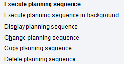
Provide the Plng Area, Pl. level, Pl. func, Param.grp, and Pl.package (Figure 30) and then select the save all icon. This new planning sequence will appear in the list of available planning sequences. Right-click on the planning sequence and select the option Execute planning sequence or Execute planning sequence in background (Figure 31).

Figure 30

Planning sequence details

Figure 31

Execute planning sequence

Key Lessons Learned on Improving Performance

This section lists some of the key lessons learned and performance improvement techniques:

1. Use the ABAP collect statement instead of the insert statement in the function module when adding a record to hashed table XTH_DATA.

2. Try to avoid doing allocations at a very detailed level as it generates too many records and the processing and validation against master data takes a long time before the data is saved to the cube.

3. Using the function module, if the cube from which data is read has aggregates built into it or if it is on SAP NetWeaver BW Accelerator, set the parameter I_USE_AGGREGATES = ‘’ in the call to function module RSDRI_INFOPROV_READ. This reads data directly from the cube but not from the aggregate or SAP NetWeaver BW Accelerator.

4. While doing year-to-date allocations, remove the calendar/year/month from the allocation level and perform the allocation at a summarized level. After the allocation data is generated, split the summarized allocation data into each month and adjust the amount according to selected criteria while loading to the reporting cube.

5. Try to run the allocations as background jobs instead of foreground jobs.

6. Since some of the allocations could be at a detailed level with intense business logic, it is a good idea to monitor the memory usage on production server(s) during the initial few runs. This   helps in catching any problems and taking corrective actions.

Allocations Done Using IP and Reusing the Function Module Used in Business Planning and Simulation

Most of the effort in creating these allocation processes in Business Planning and Simulation is in the development of the business logic in the function modules used by the planning functions. The rest of the effort is in creating cubes and planning objects. While migrating to Integrated Planning, creating Integrated Planning planning objects is minimal if you can reuse the function modules.

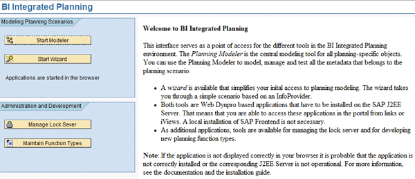
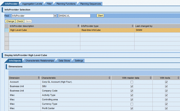
Create a real-time cube in transaction RSA1. Go to transaction RSPLAN and select the Start Modeler button (Figure 32).

Figure 32

Start the IP modeler

Provide the name of the real-time cube you created and click the Start button as shown in Figure 33. The details of the real-time cube are displayed.

Figure 33

InfoProvider details

Select the Aggregation Levels tab (Figure 34) and select the Create button.

Figure 34

Aggregation levels

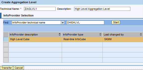
Provide the Technical Name and the Description of the aggregation level and click the Transfer button (Figure 35).

Figure 35

Create the aggregation level

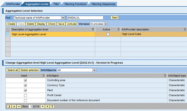
Select all the characteristics and key figures that are part of the allocation process as shown in Figure 36 by selecting the Used check boxes. Click the Save button and then the Activate button.

Figure 36

Save and activate aggregation level

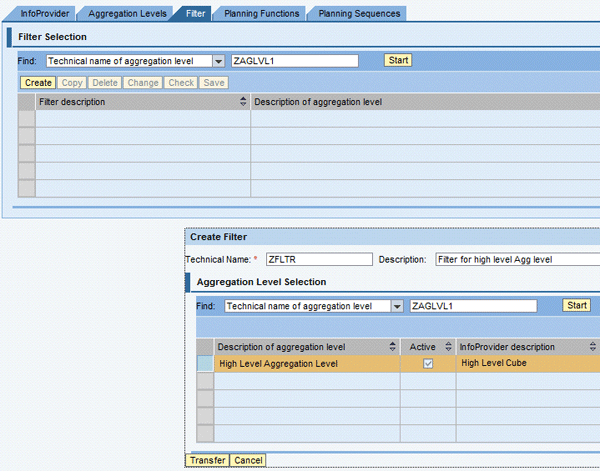
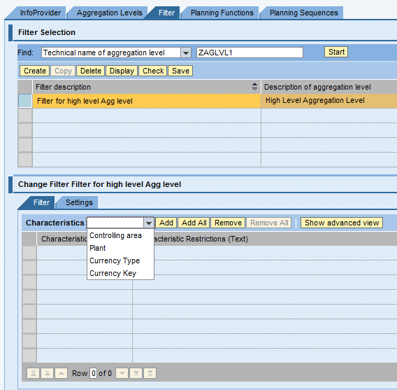
Select the Filter tab and click the Create button (Figure 37). Provide the Technical Name and the Description of the filter (Figure 37). Click the Transfer button.

Figure 37

Filter details

Select the Characteristics for which you want to add the filter criteria and click the Add button as shown in Figure 38.

Figure 38

Filter settings

For each selected characteristic in the filter use the Input Help button to provide either a fixed value or a variable value and select the Can Be Changed at Execution button if required (Figure 39). Select the Save button (Figure 38). Setting the filter values executes the allocation process on a particular data set of the cube.

Figure 39

Filter settings

The next step is the creation of the Planning Function of the type Exit and assigning the function module that has the customized logic for the allocation process. The Business Planning and Simulation functions you developed, which have customized logic written through function modules, can be reused in Integrated Planning without any interference of Business Planning and Simulation.

Integrated Planning does not provide the option of defining an Exit planning function directly on the planning modeler. To have this planning function exit type appear in the Planning Functions tab, make use of an SAP-delivered wrapper class CL_RSPLFC_BPS_EXITS.

The class forms an interface and fetches the data from the back end. It is important note that the fetched data is converted into tables that are used in the interfaces of the Business Planning and Simulation function modules. After the data is changed in the function modules, the tables are converted back to the Integrated Planning format. Therefore, Business Planning and Simulation functions are not used. Rather you call the underlying function modules.

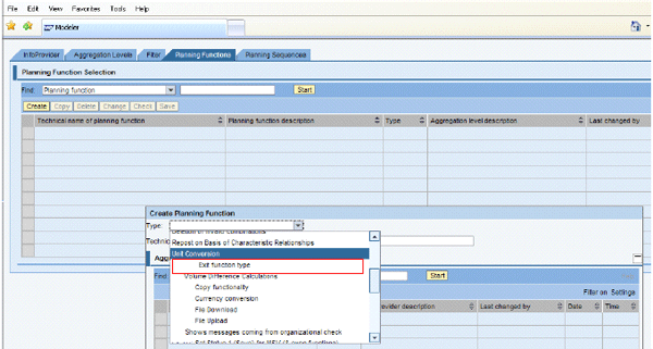
Create a Planning function type Exit function type in transaction RSPLF1 to use the functionality of the wrapper class. You create the two parameters to hold the exit and init function modules. Then the new planning function type Exit function type appears in the Planning Functions tab (planning modeler) (Figure 40).

Figure 40

Planning function types

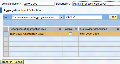
Click Exit function type and provide the technical name and description of the Planning function. Click the Transfer button (Figure 41).

Figure 41

Planning function details

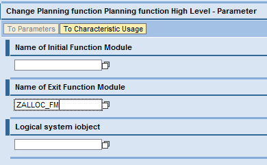
Provide the technical name of the function module that has customized allocation logic (Figure 42) and select the Save button on the Planning Functions tab (Figure 40). Note that this function module can be the same one used in Business Planning and Simulation.

Figure 42

Planning function, function module details

Note: In the step-by-step instructions of this section the aggregation level is created on a real-time cube. However, for my business scenario the aggregation level should be created on a multi-cube that has the extraction and high-level cubes as underlying cubes.

SivaKumar Bhagavatula

SivaKumar Bhagavatula is a BI technical architect at Chevron. He is an SAP NetWeaver BW-certified consultant and is heavily involved in collaborating with business partners to convert requirements to optimal technical solutions. He has more than 14 years of development and global consulting experience with SAP, Enterprise, and Internet technologies. At Chevron he is responsible for researching new technologies that are applicable for the needs of energy business. He thanks his colleagues, Archie Roberts and Clabaugh James, and his mentor, Anupam Gupta, for their support, guidance and encouragement.

You may contact the author at skmm@chevron.com.

If you have comments about this article or publication, or would like to submit an article idea, please contact the editor.