Reporting is an increasingly important factor in business operations as data continues to grow in organizations. To help address reporting challenges, organizations are looking at how to refine their data processing components and infrastructure. SAP’s chief offering to meet this need is SAP HANA, which executes analytical reports on massive data through SAP-certified hardware. This data resides in memory. Initial loads and delta replication on the HANA server with compression make it very fast for online transaction processing (OLTP) transactions.

Moreover, moving into cloud storage could provide higher flexibility, availability, and real-time (or scheduled) data sourcing from various systems. Various front-end tools can be used to fetch this data and make it available for the user to change, update, or delete. It is a foundation on which not only real-time analytics can be performed but also a set of applications can be built.

First I’ll show you how HANA’s architecture and modeling works. I’ll then provide other tips to set you on your way with HANA.

Architecture

HANA wipes out all the latency between the availability of operational data in the hands of decision makers to plan, forecast, simulate or consolidate. I’ll go through row store, column store, and engines, as covering all aspects of architectures would be too long and beyond the scope of this article. Row- and column-based storage techniques or technology are used for storing data in HANA. Each technique has its own advantages.

Indexing rows is the common way to fetch and speed up row-based table access. This works well if the query satisfies index searches, but it may increase the chance that there is a failure to read data from the cache if the query is not satisfied. Following are the characteristics of row- and column-based storage.

Row-based storage characteristics include:

1. Row-based storage is the classical means of storage and indexing.
2. When the row is inserted into the table, the indexing has to be generated to speed up the process.
3. Only a single record is required at one time.
4. Aggregation is not required and the column containing distinctive values leads to lower compression.
5. The application requires you to access a complete record instead of a whole column.

Column-based storage characteristics include:

1. Aggregation.
2. Column-based storage offers compression of data.
3. If distinctive values are present (i.e., cardinality), column-based storage is better.
4. Improves read and write functionality of delta updates.
5. Supports parallel processing.
6. The table is accessed based on columnar values rather than returning the whole row.

A quick word on compression. Compression makes it possible to fit and zip massive amounts of data in memory. Multiple CPUs share the same bus while passing data from memory to the CPUs and hence compression is quite useful. Compression must be kept in consideration. If a large amount of data is compressed then while reading the compressed data the CPU has to work on it to decompress it. After performing its tasks it should compress it again. Therefore, I recommend you start with column-based storage, and then switch to row-based storage, while keeping in mind the fifth point mentioned above for row storage.

Modeling

Modeling or data modeling is a process in which you collect all the facts or operational data of an enterprise from various sources or systems and produce graphs or reports that provide meaningful information to the business. The fact data is further linked or joined to attributes. It can also be referred to as a tool that retrieves facts and attributes from the organization and produces a set of information that is required by the management or decision makers to better understand the current market or analyze their respective business. There are different views to analyze data and before jumping into those views you need to understand the purpose of each view.

Attribute View

A simple explanation of the attribute view is that it gives context to master data tables. The attribute is called a characteristic in SAP NetWeaver BW terminology. Attribute views are reusable objects that can be consumed by several other views (e.g., attribute views or analytical views). For example, you create an attribute view of an employee including his personnel number, name, and other information to another attribute view that contains his or his family dependents’ data. Moreover, this attribute view can be joined to an analytical view, which contains employee salary, cost center, and so on. Attribute views are used to connect to the measures (also known as key figures in BW terminology) present in the fact table or analytical view to provide a meaningful view at the reporting levels through text rather than presenting numeric IDs (e.g., customer number, material number). You use a join to connect various master data tables to each other.

Analytical Views

These views leverage the computing power to calculate and aggregate transactional data and thus form the data foundation based on transactional data. You must select at least one measure and this fact table is joined against modeled data (i.e., attributes to give meaningful information to the business transactions). Aggregation for the measures must be defined using SUM, MIN, or MAX while attributes can be handled like normal columns.

Calculation Views

Calculation views can be a script calculation view or a graphical calculation view. Calculation views are created by joining various database tables, analytical views, attribute views, and calculation views, and must contain at least one measure. The results from several analytical views can be joined together using UNION to produce a result containing various analytical view outcomes.

A sequence of SQLScript that is executed to produce the calculation view is referred to as a script calculation, whereas graphical views are created through the graphical modeling features of SAP HANA Modeler.

SAP HANA Engines Overview

Engines are important to consider while modeling as they affect the performance of the view or data model designed. There are three engines particularly involved when creating views in SAP HANA Modeler:

1. Join engine (attribute view)
2. OLAP engine (analytical view)
3. Calculation engine (calculation view)

Keep in mind that an analytical view or attribute view with the calculation attribute is considered a calculation view and SAP recommends you avoid such use in general.

Now let’s look at the HANA server and start using modeling. You can request your SAP HANA Server from this link. SAP provides a 30-day evaluation period to use the HANA server. After filling out the form and related information, SAP mails you a user name, server host name, and password to let you start using the HANA Server. SAP provides information on how to log in via cloud share. Once you do that, log in and follow the steps to start working with SAP HANA.

First, create a folder. Go to File > New > Folder. Enter a folder name (Figure 1) and then you’ll deploy your SAP HANA Server instance.

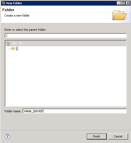
Figure 1

Folder name

Choose any name for your folder (e.g., HANA_SERVER). Now you need to add your server to it. Right-click your newly created folder and choose Add System. On the next screen, enter a Hostname and Instance Number provided to you in the mail with your user name and password (Figure 2).

Figure 2

Enter the Hostname and Instance Number values

Click the Next button and give your User Name and Password you received from SAP (Figure 3). Click Next to proceed (Figure 4). You can’t change anything here, so just click Finish.

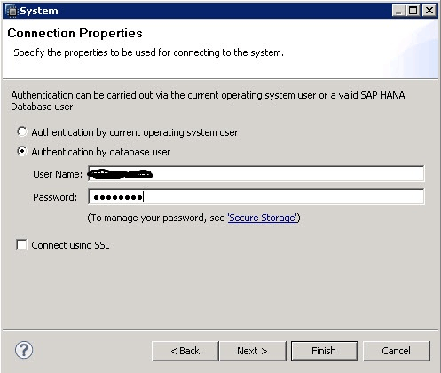
Figure 3

Enter your User Name and Password values

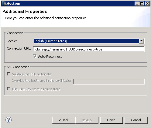
Figure 4

Click Finish

After you have added your server, you should see a screen similar to the one shown in Figure 5.

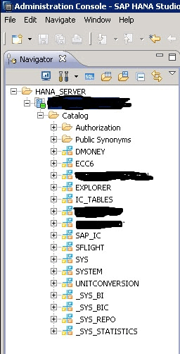
Figure 5

Catalog of your SAP HANA system

Next you need to proceed to Information Modeler, in which you create your view and consume these views in SAP BusinessObjects. Switch to Information Modeler present on the top-right corner of the screen, which opens the Quick Launch tab shown in Figure 6.

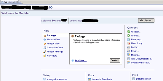
Figure 6

Information Modeler

Here you have useful links to perform modeling-related tasks, including data provisioning, managing import servers, and creating views. From the Navigator view on the left side of HANA Studio right-click Content, select New, and then choose Package… to create your own package to keep things simple and organized (Figure 7). Don’t try to use or change other users’ views or data.

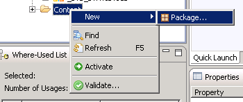
Figure 7

Add a package

Enter a meaningful name for your package and click OK (Figure 8).

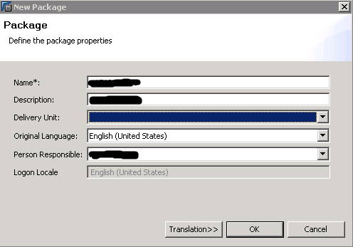
Figure 8

Package information

Now that your package is created, you are ready to create an attribute view.

Create Your First Attribute View

From the navigator view, drill down to your package, right-click it, choose New, and click Attribute View… to open the New Attribute View dialog (Figure 9). Fill out the Name and Description with a meaningful name and description. For this example, use this view in the analytical view as well.

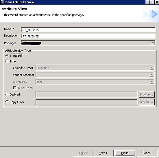
Figure 9

Input attribute view name and description

There are four types of attribute views:

1. Standard. Choose this option if you want a plain attribute view in which you can put some tables and join them to provide meaningful information.
2. Time. This view is worth choosing when you want to see data using fiscal calendars and need them to be aligned in accordance with the calendar. It is best to choose it when you have different calendars or fiscal periods that are not aligned with the calendar.
3. Derived. You can use attribute views more than once in other views, and this view lets you incorporate them. You can start building your own on top of a derived model. The derived model is read only and you are allowed to change only its description.
4. Copy From. This allows you to copy an attribute view.

Click the Next button to proceed (Figure 10).

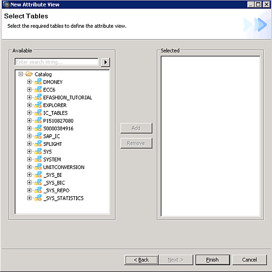
Figure 10

Select tables for your attribute view

As examples, I’ll show you attribute views in action with SBOOK, SCARR, and SCUSTOM. Go through the tree or search for your specific table. You can add any table from any package. It’s not necessary that the tables should be in the same package but they can be in different packages.

After clicking the Add button, click the Finish button (Figure 11).

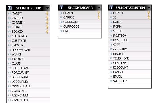
Figure 11

Tables in an attribute view

Now that your required tables are added to the attribute view you need to consider how to join these tables. There are multiple types of joins to consider while modeling. Every join has its own benefit.

1. Text join. This join is used to give a meaningful return or value to your data as it is joined to the master table. Text joins act as left outer joins and can be used with SAP tables in which you have a language column.
2. Inner join. By default this is your join. If both values match in both tables, those records are available.
3. Left outer join. The best use for this join is in the analytical view. It takes all the records from the left table, even if there is no matching key or figure to the joined table.
4. Right outer join. This is just the opposite of the left outer join, where all records from the right table are picked even if there is no matching figure on the left table.
5. Full outer join. A full outer join returns all rows from the left and right tables. It includes all records from the left table as well as the right table and non-matching values return NULL values.
6. Referential join. Referential integrity is optimized for performance. It is semantically an inner join that assumes that referential integrity is given, which means that the left table always has a corresponding entry on the right table. It is actually faster than any other join, where the right table is not checked if no data is requested from the right table. It best fits in a scenario in which you are sure that each record in a table has a joining row in the other table and goes from the left side to the right side.

Select a couple of fields from these derived tables to be viewed and consumed in the attribute view. There are two types of attributes you can select: key attribute and attribute. Attributes work as normal attributes and key attributes are unique keys to identify particular records. Add CARRID (carrier ID) as a Key Attribute (Figure 12).

Figure 12

CARRID has been added as Key Attribute

You can add any number of attributes in Attribute view but there should always be at least one key attribute. Now you need to join these tables (Figure 13).

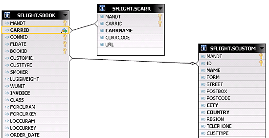
Figure 13

Join the tables in the attribute view

See those bold fields in the tables. They are added as attributes to the attribute view. Save and validate, and then activate this view by clicking the activate icon  on the top-right corner of the screen to view the initial output. The view is automatically saved and activated to be consumed by other views. In case of errors, you can jump into the error log, which can give you a complete description of what has caused this error. You see the Completed Successfully message in the job log window if it is successfully activated.

Right-click your view in the Navigator window and choose Data Preview to see this view in action.

Analytic View

To start creating an analytic view, you can jump to the Quick Start page or right-click your package and choose New > Analytical View (Figure 14). This brings up the screen in Figure 15.

Figure 14

Create an analytic view

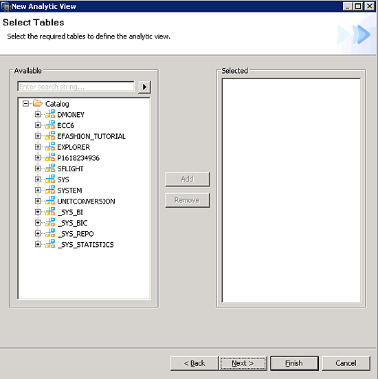
Figure 15

Select tables for the analytic view

Now choose tables for your analytic view. Later, you select measures from the tables. Either choose a table from the tree view or search for it. It is also possible to select the tables at a later stage by drag and drop. For the purposes of this article, I select the table SNVOICE and click the Next button to proceed (Figure 16).

Figure 16

Choose Attribute View for this analytic view

Select Dimensions (Attribute View) if you need to include them at this stage. You can add an attribute view at a later stage also, which is illustrated in this article. Click the Finish button to exit. Now you can see the Data Foundation (Figure 17).

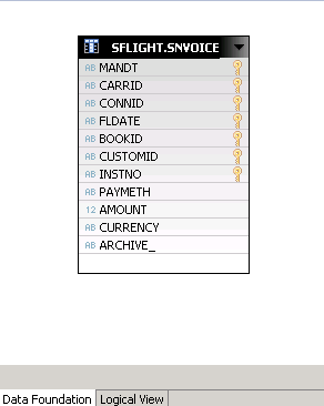
Figure 17

Data Foundation

Select a measure and then in the logical view bind it to your dimensions to give it meaningful information. Right-click CARRID, CONNID, and BOOKID, and choose Add As Attribute. You want to do this because you need to connect it to your dimension, AT_FLIGHTS. Remember, you need to have at least one attribute and measure in your analytic view.

After adding them, right-click the AMOUNT field and choose Add As Measure (Figure 18).

Figure 18

Analytic view data foundation

Switch to the logical view, in which you connect or join the attribute view to your fact table. Drag and drop your previously created attribute view (Figure 19).

Figure 19

Logical View

In this example, AT_FLIGHTS (attribute view) is added to the logical view and now you need to join them to your fact table. Select all key attributes of the attribute view to join them. By default the join is an inner join. You can add as many attribute views here that are in contrast to these fact tables. Drag and drop CARRID, CONNID, and BOOKID on top of the same fields present in the Data Foundation (Figure 20).

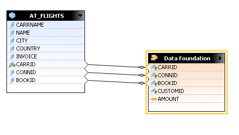
Figure 20

Joining the attribute view to Data Foundation

Save and activate. Right-click AN_FLIGHTS (Analytical View) from the Navigator window on your left side and choose Data Preview. You are presented data in raw format. Choose the Analysis tab on top of the screen. For Labels axis select CARRNAME and for the Values axis select AMOUNT (Sum) (Figure 21).

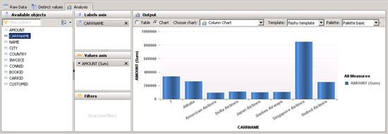
Figure 21

Testing analytic view

Muhammad Usman Malik

Muhammad Usman Malik is a senior SAP consultant at Saudi Business Machines (SBM), Saudi Arabia. Usman has been involved in ABAP development and functional configuration of HR for many years. He has several years of experience implementing and supporting SAP systems including logistics, WebDynpro ABAP, workflow, and FI/CO at multinational and local companies.

You may contact the author at usman.malik.sap@gmail.com.

If you have comments about this article or publication, or would like to submit an article idea, please contact the editor.