Learn the configuration, use, and importance of proportional factors. See how they can be used to control the disaggregation of values in SAP Advanced Planning and Optimization (SAP APO) Demand Planning (DP). Follow a step-by-step procedure to configure and run the associated master data objects, run simulations, and interpret the results.
Key Concept
Demand Planning (DP) in SAP Advanced Planning and Optimization (SAP APO) is used to carry out forecasting using different statistical algorithms. It helps to carry out consistent planning at all levels. Aggregation is used to sum the values at a detailed level and show or carry out planning at an aggregate level. Disaggregation is the drill-down or breakup of values from the aggregate to a detailed level. Both aggregation and disaggregation of data help to carry out consistent planning across all levels. Values in key figures are always stored and saved at the lowest level.
SAP Advanced Planning and Optimization (SAP APO) Demand Planning (DP) is based on the concept of consistent planning across all levels. It means that if you look at the data at the aggregate level, values at the detailed level are summarized in real time. In other words, any change at the aggregate level is automatically disaggregated down to the detailed level in real time. It helps in providing a consistent and stable view of data from all directions.
Proportional factors in SAP APO allow you to disaggregate data from the aggregate level to a detailed one. Use of proportional factors in DP provides businesses with the flexibility to decide which rules to use to control the disaggregation process. For example, suppose a television (TV) manufacturer sells different models of TVs in different regions, and each region has different customers. Past sales history can be used to forecast future sales data. The aggregation level to carry out forecasting depends on the business requirement — for example, product or location. If the forecast is executed at the product-location level, it needs to be further disaggregated down to a lower level — for example, customers. This level of disaggregation can be controlled by the proportional factors by deciding which method and what proportions to use.
Overview of the Disaggregation Mechanism and Use of Proportional Factors
All data that can be represented as numerical values is stored in key figures. Settings in the calculation type of the key figure determine how values are aggregated and disaggregated. The settings are valid for all planning books in which key figures are used. Figure 1 shows the high-level classification of different structural disaggregation methods present in SAP APO. Although there are other methods such as D (average at the lowest level), they are variants and depend on these more general methods. For discussion in this article and to show the calculation via proportional factors, I focus on the methods S and P.
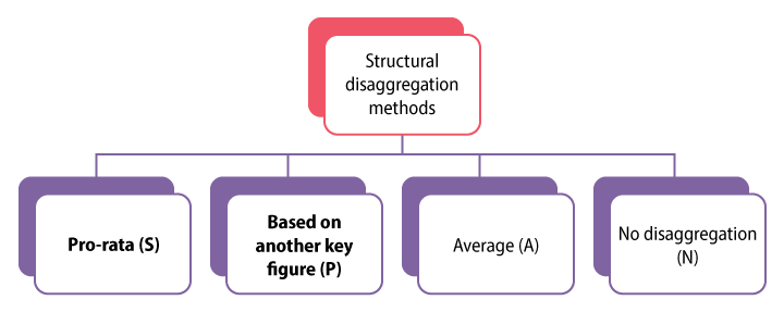
Figure 1
High-level classification of structural disaggregation methods
Configuration in DP
Before using proportional factors, you need to set up a few DP objects. I assume that you know how to set up master data in SAP APO and how to configure basic DP objects. For this article, I show screenprints of the important DP objects highlighting configurations specific to proportional factor calculation. My focus is on explaining how calculations are done and how to interpret the results.
Master Planning Object Structure (MPOS)
An MPOS is created via transaction code /SAPAPO/MSDP_ADMIN. For the example discussed in this article, the MPOS contains the Location, Product, Product Group, and Customer as shown in Figure 2.
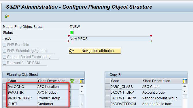
Figure 2
An MPOS
Planning Area
A Planning Area is created via transaction code /SAPAPO/MSDP_ADMIN. Planning Areas are based on the MPOS shown in above step (i.e., ZNEW). A Planning Area contains key figures related to forecast and history as shown in Figure 3. Note that the calculation type of the Corrected Forecast key figure is P (i.e., based on another key figure) and the disaggregation key figure is APODPDANT. The system stores the proportional factors internally in the key figure APODPDANT. The calculation type of other key figures is S (i.e., pro-rata). I explain the difference between these two calculation types later in the article.
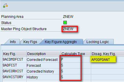
Figure 3
The Planning Area
Planning Book
To create a Planning Book use transaction code /SAPAPO/SDP94. The Planning Book is based on the Planning Area created in the above step (i.e., ZNEW). Note that when you create a Planning Book, you need to select the Manual Proportion Maintenance check box, as shown in Figure 4. After you select this check box, you can manually edit proportional factors in interactive planning. For my example, select the Univariate forecast check box as it is needed for forecasting but it is not specific to proportional factors.
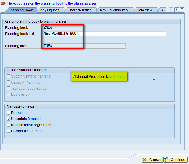
Figure 4
The main screen of the Planning Book
Now you need to assign the internal key figure for the proportional factor calculation (i.e., APODPDANT) to a data view in the Planning Book. Figure 5 shows that key figure Proportional Factor is assigned to the Data View for this Planning Book.
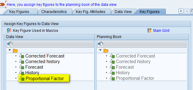
Figure 5
Key figure assignment to the Data View in the Planning Book
Characteristic Value Combinations (CVCs)
To create a CVC use transaction code /SAPAPO/MC62. Figure 6 shows the list of CVCs that are assigned to the Planning Area used in this article.
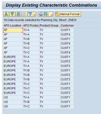
Figure 6
The CVC list
Interactive Planning Book
You access an interactive Planning Book via transaction code /SAPAPO/SDP94. For my example, load data for the AP region. Figure 7 shows the value of the key figure Corrected history for January and February 2016.
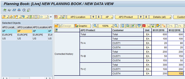
Figure 7
Values loaded in the Planning Book
Running a Simulation for Fixed Proportional Calculations and Interpreting the Results
To run a proportional factor calculation, execute transaction code /SAPAPO/MC8V. In the next screen (Figure 8), enter the name of the Planning Area (e.g., ZNEW) and the name of the Planning Area based on the proportional factor you want to calculate (i.e., ZNEW). Click the execute icon.
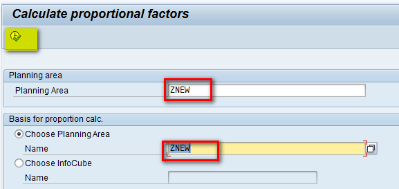
Figure 8
The Calculate proportional factors main screen
Enter the parameters highlighted in Figure 9.
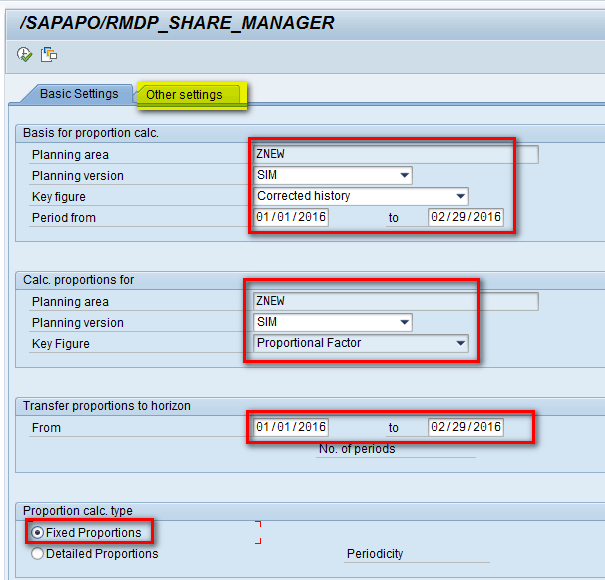
Figure 9
Basic settings for the proportional factor
For my example, calculate the proportional factor for January and February 2016. The basis for the proportional factor calculation is the key figure Corrected history using the values shown in Figure 7. The results are stored in the key figure proportional factor (i.e., APODPDANT). After entering the values, click the Other settings tab (Figure 10).
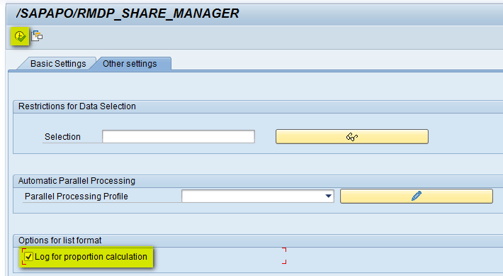
Figure 10
Other settings for proportional factors
In Figure 10, select the Log for proportion calculation check box and then click the execute icon.
For a fixed proportion calculation, the system first calculates the total value of the key figure for all CVCs for all periods in the specified horizon. It then sums the key figure value for all CVCs in the entire horizon and determines the proportion of each individual CVC in the total CVC list. Figures 11 to 13 show the log results. They are the common logs generated after you click the execute icon in Figure 10. Compare the values in Figures 11 to 13 and note that the calculation happens as per Table 1.
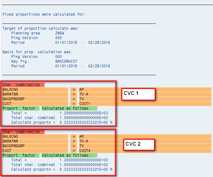
Figure 11
Fixed proportion calculation log 1
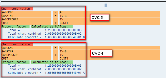
Figure 12
Fixed proportion calculation log 2
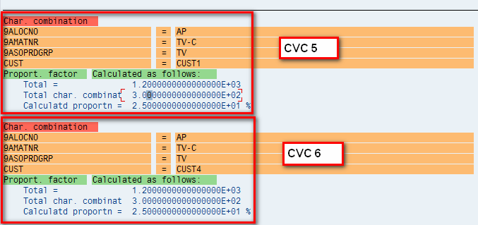
Figure 13
Fixed proportion calculation log 3
Note
Figures 11 to 13 show the results in one log, but I have separated these results into three separate figures.
To complete a proportional factor calculation based on the values shown in Table 1, follow, use the SAP system to complete these steps:
- Calculate the sum of key figure Corrected history for January and February 2016 for all CVCs (i.e., 600 + 600=1200)
- Calculate the sum of the key figure Corrected history for January and February 2016 for CVC1 (i.e., 20+80=100)
- Divide the value calculated in step 2 by the value in step 1 to obtain the proportion (i.e., 100/1200 = 0.0833 = 8.33 percent)
- The same steps are repeated for remaining CVCs.
|
Jan |
Feb |
Sum |
Proportion
|
Value in %
|
Total
|
600 |
600 |
1200 |
|
|
| CVC1 |
20 |
80 |
100 |
100/1200 |
8.33 |
| CVC2 |
80
|
20 |
100 |
100/1200 |
8.33 |
| CVC3 |
50 |
150 |
200 |
200/1200 |
16.67 |
| CVC4 |
150 |
50 |
200 |
200/1200 |
16.67 |
| CVC5 |
100 |
200 |
300 |
300/1200 |
25 |
| CVC6 |
200 |
100 |
300 |
300/1200 |
25 |
Table 1
Fixed proportional factor calculation
The values calculated by the system as per log messages are the same as what is calculated manually as shown in Table 1.
To check the values in the Planning Book, use transaction code /SAPAPO/SDP94 and load the data in the Planning Book. You can see that values in the proportional factor key figure are the same as what was calculated by the system, as shown in Figure 14.
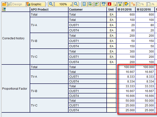
Figure 14
Fixed proportional results in the Planning Book
Now you know that the key figure Corrected Forecast has Calculation Type P (i.e., based on the Proportional Factor key figure as shown in Figure 3). You also have values calculated in the proportional factor for all CVCs in January and February 2016. To see how these proportional values are used during disaggregation, enter values at the aggregate level for the Corrected Forecast key figure (e.g., 600 and 900) as shown in Figure 15. Press Enter.
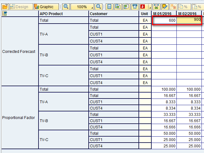
Figure 15
Values at the aggregate level for the corrected forecast
After you press Enter, the total values at the aggregate levels of 600 and 900, respectively, are disaggregated among the six CVCs. Also the ratio in which they are disaggregated is based on the values present in the Proportional Factor key figure. For example, Product TV-A and Customer-CUST1 have a proportional factor of 8.33 percent in January and February 2016, so 8.33 percent of 600 (i.e., 50) and 8.33 percent of 900 (i.e., 75) are the calculated values. A similar calculation is done for other CVCs. The values are as shown in Figure 16.
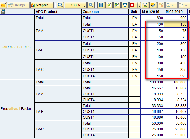
Figure 16
Values at a detailed level for the corrected forecast
Table 2 shows the calculation that was done by the system to calculate the values highlighted in bold type. These are the same values shown in the red box in Figure 16.
|
Jan |
Feb |
Calculation — Jan |
Calculation — Feb |
Result — Jan |
Result — Feb |
Total
|
600
|
900
|
|
|
|
|
CVC1
|
8.33
|
8.33
|
8.33% of 600 |
8.33% of 900 |
50 |
75 |
CVC2
|
8.33
|
8.33
|
8.33% of 600 |
8.33% of 900 |
50 |
75 |
CVC3
|
16.66
|
16.66
|
16.66% of 600 |
16.66% of 900 |
100 |
150 |
CVC4
|
16.66
|
16.66
|
16.66% of 600 |
16.66% of 900 |
100 |
150 |
CVC5
|
25
|
25
|
25% of 600 |
25% of 900 |
150 |
225 |
| CVC6 |
25 |
25 |
25% of 600 |
25% of 900 |
150 |
225 |
Table 2
Disaggregation calculation using fixed proportional factor values
Running a Simulation for a Detailed Proportional Calculation and Interpreting the Results
Now calculate the proportional factor using the detailed proportions calculation method. For the calculation, use the same values of Corrected history as defined in Figure 7. To calculate the proportional factor, execute transaction code /SAPAPO/MC8V. In the next screen enter the same parameters that were defined while running the fixed proportional calculation. The only difference here is that I have selected the Detailed Proportions radio button as highlighted in Figure 17. Then click the Other settings tab (Figure 18).
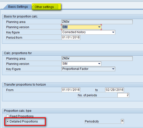
Figure 17
Basic settings for the proportional factor
In Figure 18 you can see that there is no option for generating the log messages, which was the case while calculating the fixed proportion as shown in Figure 10. This option, the Log for proportion calculation check box, is only visible when the proportional factor is calculated for the same planning area if:
- Fixed factors are being calculated
- No parallel processing profile has been entered
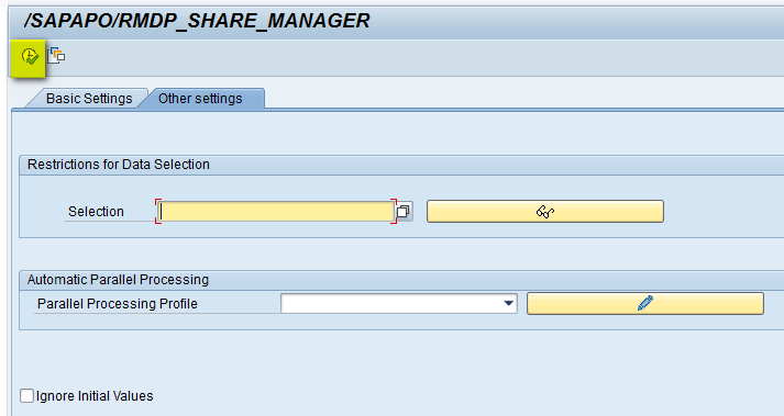
Figure 18
The Other settings tab for the proportional factor
Click the execute icon as shown in Figure 18.
For a detailed proportion calculation, the system first calculates the total value of the key figure for all CVCs for each period in the specified horizon. It then calculates the proportion of each CVC per period. The calculation happens as shown in Table 3.
Here are the steps that explain how to use the SAP system to complete the steps for the example:
- Calculate the sum of key figure Corrected history for January 2016 for all CVCs (i.e., 600).
- Identify the value of the of the key figure Corrected history for January 2016 for CVC1 (i.e., 20).
- Divide the value calculated in step 2 by the value in step 1 to obtain the proportion (i.e., 20/600=0.0333=3.33 percent).
- The same steps are repeated for the remaining CVCs for January 2016.
- The same steps are repeated for all CVCs in February 2016.
To check the values in the Planning Book, execute transaction code /SAPAPO/SDP94. In the screen that appears (Figure 19) load the data in the Planning Book. You can see that values in the proportional factor key figure are the same as what was calculated in Table 3 as shown in Figure 19.
|
Jan |
Feb |
Calculation — Jan |
Calculation — Feb |
Result — Jan (in %) |
Result — Feb (in %)
|
Total
|
600
|
600
|
|
|
|
|
CVC1
|
20
|
80
|
20/600
|
80/600
|
3.33 |
13.33 |
CVC2
|
80
|
20
|
80/600
|
20/600
|
13.33 |
3.33 |
CVC3
|
50
|
150
|
50/600
|
150/600
|
8.33 |
25 |
CVC4
|
150
|
50
|
150/600
|
50/600 |
25 |
8.33 |
CVC5
|
100
|
200
|
100/600
|
200/600
|
16.66 |
3.33 |
| CVC6 |
200
|
100
|
200/600
|
100/600
|
33.33 |
16.66 |
Table 3
Detailed proportional factor calculation
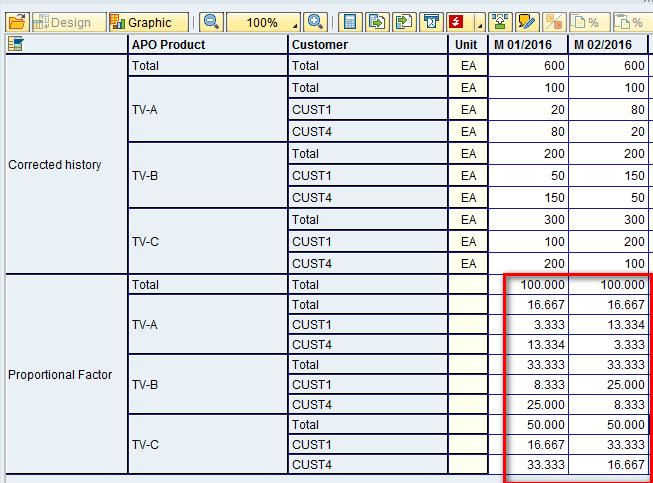
Figure 19
Detailed proportional results in the Planning Book
Now you know that the key figure Corrected Forecast has Calculation Type P (i.e., based on the Proportional Factor key figure shown in Figure 3). You also have values calculated in the proportional factor for all CVCs in January and February 2016. To see how these proportional values are used during disaggregation, enter values at the aggregate level for the Corrected Forecast key figure (e.g., 600 and 1200) as shown in Figure 20 and then press Enter. (Note the earlier values in the Corrected Forecast key figure are deleted so that the calculation happens in accord with the new proportional factor values.)
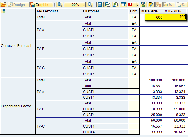
Figure 20
Values at the aggregate level for the corrected forecast
After you press Enter, the total values at the aggregate level (i.e., 600 and 900, respectively) are disaggregated among all six CVCs. The ratio in which they are disaggregated is based on the values present in the Proportional Factor key figure. For example Product TV-A and Customer CUST1 have a proportional factor of 3.33 percent in January 2016, so 3.33 percent of 600 (i.e., 20) is the calculated value. A similar calculation is done for other CVCs and the values are as shown in Figure 21.
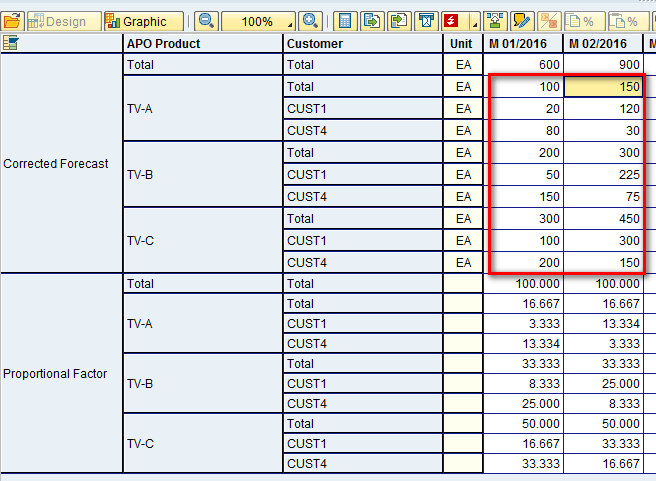
Figure 21
Values at a detailed level for the corrected forecast
Table 4 shows the calculation that is done by the system to calculate the values highlighted in bold type. These are the same values shown in the red box in Figure 21.
|
Jan |
Feb |
Calculation — Jan |
Calculation — Feb |
Result — Jan |
Result — Feb
|
Total
|
600
|
900
|
|
|
|
|
CVC1
|
3.33
|
13.33
|
3.33% of 600
|
13.33% of 900
|
20
|
120
|
CVC2
|
13.33
|
3.33
|
13.33% of 600
|
3.33% of 900
|
80
|
30
|
CVC3
|
8.33
|
25
|
8.33% of 600
|
25% of 900
|
50
|
225
|
CVC4
|
25
|
8.33
|
25% of 600
|
8.33% of 900
|
150
|
75
|
CVC5
|
16.66
|
33.33
|
16.66% of 600
|
33.33% of 900
|
100
|
300
|
| CVC6 |
33.33
|
16.66
|
33.33% of 600
|
16.66% of 900
|
200
|
150
|
Table 4
Disaggregation calculation using detailed proportional factor values
Running a Simulation for Manual Proportional Maintenance and Interpreting the Results
In the above two sections, “Running a Simulation for Fixed Proportional Calculations and Interpreting the Results” and “Running a Simulation for a Detailed Proportional Calculation and Interpreting the Results,” you saw how proportional factors were calculated by the system using two different methods — fixed and detailed. Instead of using the calculated values, you also can go in the Interactive Planning Book manually to edit the proportional factor values. To change the proportional factor values, navigate to the Interactive Planning Book using transaction code /SAPAPO/SDP94. Enter the values of the proportional factor for all six CVCs as shown in Figure 22.
Figure 22
Manual maintenance of proportional factor values
To see how these proportional values are used during disaggregation, enter values at the aggregate level for the Corrected Forecast key figure (e.g., 600 and 900) as shown in Figure 23 and then press Enter.
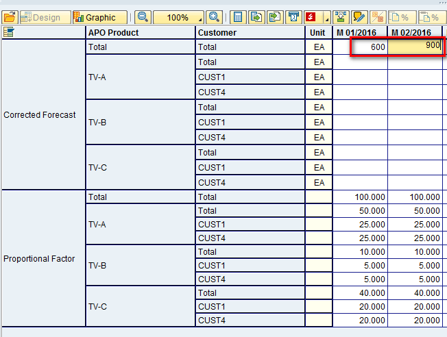
Figure 23
Values at the aggregate level for the corrected forecast
After you press Enter, the total values at the aggregate level are disaggregated among all the six CVCs. Also the ratio in which they are disaggregated is based on the values present in the Proportional Factor key figure. For example Product TV-A and Customer CUST1 have the proportional factor of 25 percent in January and February 2016, so 25 percent of 600 (i.e., 150) and 25 percent of 900 (i.e., 225) are the values calculated. A similar calculation is done for other CVCs. The values are shown in Figure 24.
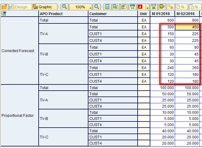
Figure 24
Values at a detailed level for the corrected forecast
Table 5 shows the calculation done by the system to calculate the values highlighted in yellow. These are the same values shown in the red box in Figure 24.
|
Jan |
Feb |
Calculation — Jan |
Calculation — Feb |
Result — Jan |
Result — Feb
|
Total
|
600
|
900
|
|
|
|
|
CVC1
|
25
|
25
|
25% of 600
|
25% of 900
|
150
|
225
|
CVC2
|
25
|
25
|
25% of 600
|
25% of 900
|
150
|
225
|
CVC3
|
5
|
5
|
5% of 600
|
5% of 900
|
30
|
45
|
CVC4
|
5
|
5
|
5% of 600
|
5% of 900
|
30
|
45
|
CVC5
|
20
|
20
|
20% of 600
|
20% of 900
|
120
|
180
|
| CVC6 |
20
|
20
|
20% of 600
|
20% of 900
|
120
|
180
|
Table 5
Disaggregation calculation using manual proportional factor values
Differences Between Pro-Rata Disaggregation and Disaggregation on Another Key Figure
Based on the calculation type of the key figures defined in Figure 3, you know that the Forecast key figure has the calculation type S (i.e., pro-rata).
Scenario 1 – Data Created at the Aggregate Level
To understand how values are disaggregated using calculation type S, execute transaction code /SAPAPO/SDP94. Delete any existing values (if any) in the Forecast key figure. Now enter the values of 600 and 900 for January and February 2016, respectively, as shown in Figure 25. Press Enter.
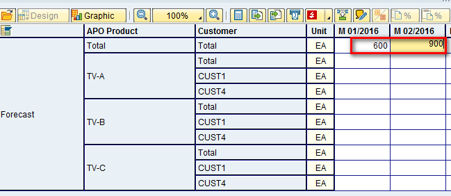
Figure 25
Values at the aggregate level for the forecast key figure
After you press Enter, values are disaggregated among all six CVCs. Because data is created at the aggregate level, it is distributed to the lowest level in equal proportions. It means the value of 600 and 900 will be equally distributed among all six CVCs. Therefore, the value of each CVC for January 2016 will be 100 (i.e., 600/6 = 100), and the value of each CVC for February 2016 will be 150 (i.e., 900/6 = 150). You can see the same values in Figure 26.
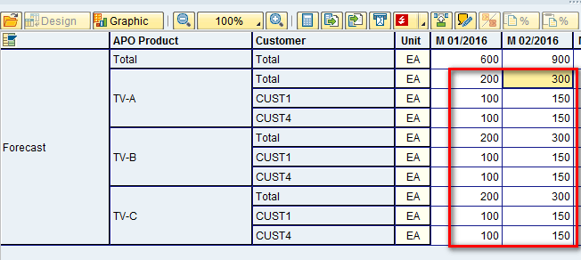
Figure 26
Values at the detailed level for forecast key figure in equal proportion
Scenario 2: Data Changed at the Detailed Level
In the same screen as the one shown in Figure 26, change the value at the detailed level for any one CVC. I changed the value of the product TV-C and customer CUST-1 combination for January 2016 from 100 to 200. Because I am changing the value at the detailed level, to maintain consistency, the value at the aggregate level also increases from 600 to 700 (increase in 100 quantity) as shown in Figure 27. The system makes the change automatically.
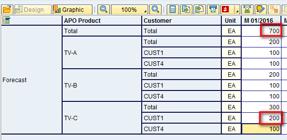
Figure 27
Values changed at the detailed level for the forecast key figure
Scenario 3: Data Changed at the Aggregate Level
Continuing with the same example, I change the data at the aggregate level from 700 to 1400 in January 2016 and then press Enter as shown in Figure 28.
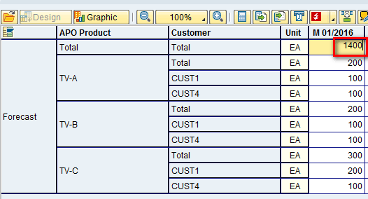
Figure 28
Values changed at the aggregate level for the forecast key figure
The system again disaggregates this value among all six CVCs. However, this time disaggregation happens such that each of the values at the detailed level represent the same proportion of the aggregate values as before. Table 6 shows how the calculation is carried out by the system internally.
|
Jan |
Proportion
|
Proportion value (%) |
Calculation
|
Value
|
Total
|
700
|
|
|
1400 |
|
CVC1
|
100
|
100/700
|
14.29
|
14.29% of 1400
|
200
|
CVC2
|
100
|
100/700
|
14.29
|
14.29% of 1400
|
200
|
CVC3
|
100
|
100/700
|
14.29
|
14.29% of 1400
|
200
|
CVC4
|
100
|
100/700
|
14.29
|
14.29% of 1400
|
200
|
CVC5
|
200
|
200/700
|
28.57
|
28.57% of 1400
|
400
|
| CVC6 |
100
|
100/700
|
14.29
|
14.29% of 1400
|
200
|
Table 6
Disaggregation pro-rata calculation
After you press Enter in the Planning Book, the values are disaggregated as shown in Figure 29. Note that the values in the Planning Book for all six CVCs are the same as those calculated and shown in Table 6.
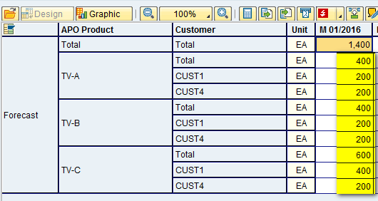
Figure 29
Values at the detailed level for the forecast key figure as per the proportional factor
Note the difference in the system behavior between scenarios 1 and 3. In scenario 1, the system disaggregates the values in equal proportion among all CVCs, whereas in Scenario 3, the system disaggregates the values in the same proportion of the aggregate values as before.
Automation and Recommendations within Proportional Calculation
In the previous section, you saw how proportional factors can be used to control disaggregation of values using various techniques. A few options are available for faster performance and automation for proportional calculation. I describe these options in this section.
Running the Proportional Factors Calculation in Background Mode
Proportional factors calculation can be run as a background job. This is important if there is an enormous number of CVCs for which calculation needs to be done. To schedule the proportional factors calculation as a background job, use program /SAPAPO/RMDP_SHARE_MANAGER. This program can be scheduled to run using the scheduling system used by a business as needed.
Running Proportional Factors Calculation in Process Chain
You can also have the proportional factor calculation as part of the process chain step. To include the step for proportional factor in a process chain, execute transaction code RSPC and under SCM – Demand Planning, there is an option for Calculate proportional factors, as shown in Figure 30, that you can use in a process chain.
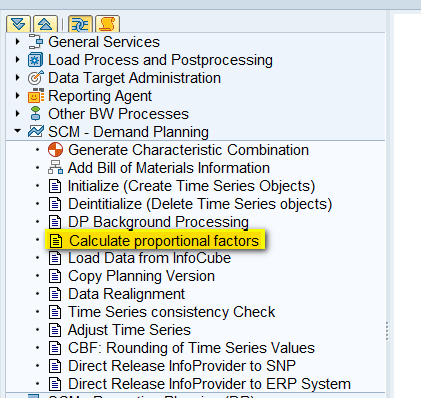
Figure 30
Proportional factors in the process chain
Use of Parallel Processing
Parallel processing is used to define how background jobs are split into parallel processes, which in turn help in faster execution of jobs. To define the parallel processing, follow menu path SPRO > APO > Supply Chain Planning > Demand Planning > Profiles > Define Parallel Processing Profile. In the screen that appears click the New Entries button (Figure 31).

Figure 31
New entries for parallel processing
In the next screen, enter the parameters as shown in Figure 32 and then click the save icon. For my example, define the number of parallel processes as 3. When the system executes the proportional factor job, three parallel processes can run simultaneously to calculate the proportional factors.
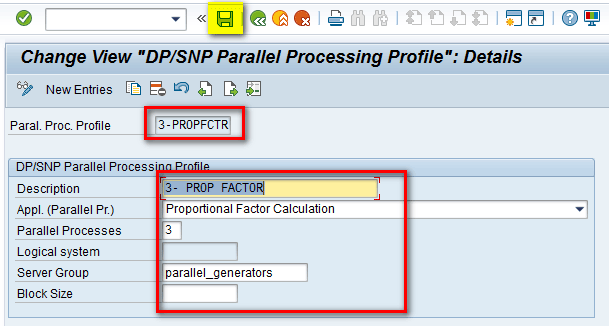
Figure 32
Parallel processing profile defined
To use the defined parallel processing profile, execute transaction code /SAPAPO/MC8V. In the Other settings tab (Figure 33), you can see that the Parallel Processing Profile field is populated (e.g., 3-PROP FACTOR) with the name of a profile. This name is the same profile defined in Figure 32.
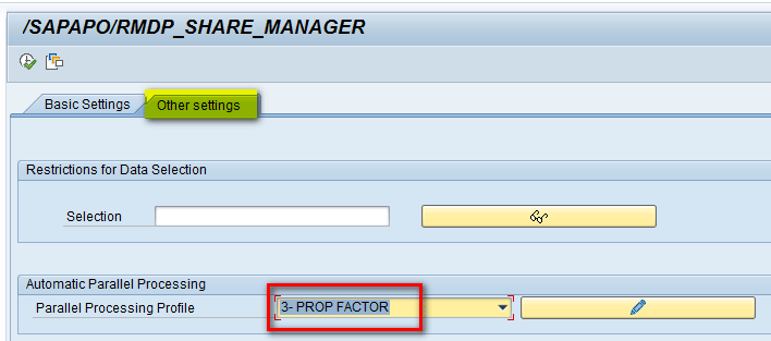
Figure 33
Parallel processing profile used in the proportional factor
Alok Jaiswal
Alok Jaiswal is a consultant at Infosys Limited.
He has more than six years of experience in IT and ERP consulting and in supply chain management (SCM). He has worked on various SAP Advanced Planning and Optimization (APO) modules such as Demand Planning (DP), Production Planning/Detailed Scheduling (PP/DS), Supply Network Planning (SNP), and Core Interface (CIF) at various stages of the project life cycle.
He is also an APICS-certified CSCP (Certified Supply Chain Planner) consultant, with exposure in functional areas of demand planning, lean management, value stream mapping, and inventory management across manufacturing, healthcare, and textile sectors.
If you have comments about this article or publication, or would like to submit an article idea, please contact the editor.