Learn about the key considerations in designing processes for measuring forecast accuracy. See how forecast accuracy reports can be implemented using SAP APO Demand Planning (DP) and SAP Business Warehouse (BW).
Key Concept
Forecast accuracy is a measure of the difference between a prediction and what actually happens. It is a crucial metric in any enterprise that performs a demand planning function. Defining a well-structured measurement process is critical to improve not only forecast accuracy but also the demand-planning process itself. As the adage goes, you cannot improve what you don’t measure.
From a business perspective, several questions to consider are:
- Which metrics should be used?
- What are the advantages and limitations of these metrics?
- At what aggregation level should the metrics be measured?
- What forecast types (such as statistical or consensus) should be measured?
- What lag, horizon, or buckets to consider? (We define lag as the number of periods before the actual demand the forecast has been generated — for example, a three-week lag is the forecast that is generated this week for three weeks out. Horizon as used in this article is the period of time over which to average accuracy metrics for reporting. Buckets identify the time granularity used for measuring forecast accuracy - for example, weeks or months.).
- Should you measure forecast accuracy in units or dollars?
From a technology perspective, consider the following:
- How do you capture sales history?
- How do you capture historical (versioned) forecasts so that lagged accuracy can be measured?
- How do you provide users with flexible yet quick report output?
We first discuss the critical business considerations and questions that need to be answered with respect to the forecast accuracy measurement process. We also describe how such a forecast accuracy measurement process can be implemented using SAP Advanced Planning and Optimization (APO), SAP Demand Planning (DP), and SAP Business Warehouse (BW). That includes high-level architecture as well as specific tricks to version forecasts, measure forecast lag, and calculate accuracy metrics using SAP BW queries.
Note
SAP Business Warehouse (BW) is a software component that SAP delivers as a part of the SAP NetWeaver platform. In this article we use the term APO BW to refer to the embedded BW component of an APO system. We use the term Enterprise BW to refer to the SAP BW system used as an Enterprise Data Warehouse for enterprise wide analytics and reporting. We use the term ‘BW Queries’ to refer to the reporting queries developed in the Query Designer feature of Enterprise BW.
Introduction to Demand Planning
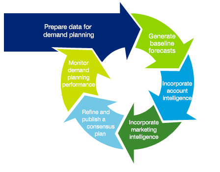
Demand planning is an iterative process that typically goes through the steps shown in Figure 1.

Figure 1
Demand planning steps
The final step is to monitor demand planning performance. This step includes the following tasks:
- Measure accuracy or error and bias of each input
- Conduct root cause analysis to determine key causes of error
- Identify and document resolution and incorporate into future forecast cycles
Need to Measure Forecast Accuracy in the Demand-Planning Process
The most important rule of forecasting is that forecasts are always wrong. However, forecast accuracy is a key driver of operational excellence and implementing broad processes for measuring forecast accuracy is crucial for two reasons:
- Forecast accuracy is an indicator of the reliability of the forecast and is a guide for upstream supply chain processes such as safety stock planning, supply planning, inventory policies, capacity planning, and vendor agreements.
- Measuring forecast accuracy can help you improve your demand planning process itself by identifying sources of forecast error such as outlier correction, incorrect statistical models, and human bias. It also can help you identify value added by each of the inputs into the demand planning process — statistical forecasts, sales overrides, or marketing overrides.
Forecast Accuracy Metrics
Because forecasting is typically done for hundreds or thousands of products over several buckets of time (weeks, months or years), statistical methods are employed to generate representative accuracy metrics. The quality of a forecast typically has two measures: bias and accuracy. Forecast bias is a measure of whether you are consistently over- or under-forecasting. It is typically calculated using the Mean Forecast Error (MFE) metric shown in Figure 2.

Figue 2
The MFE metric
Bias is a useful measure of forecast quality because it can indicate the direction of error (e.g., is the sales function consistently providing higher estimates in order to buffer customer service levels?). Forecast accuracy measures how accurate the forecast is. It is typically calculated using either of two metrics: mean absolute deviation (MAD) or mean absolute percentage error (MAPE). MAD measures the average absolute deviation of forecast from actuals as shown in Figure 3.

Figure 3
The MAD metric
MAD measures absolute error and positive and negative errors do not cancel out (as with MFE). One of the limitations of the MAD metric is that because it is an absolute number, there is no way to know if the MAD error is large or small in relation to the actual data. Therefore, it is difficult to compare accuracy across product lines or business units using this metric. This advantage is overcome by another metric called Mean Absolute Percentage Error (MAPE) that we discuss subsequently.
MAPE measures the average absolute error as a percentage of actuals as shown in Figure 4.

Figure 4
The MAPE metric
One limitation of MAPE is that combinations (product/ customer/locations/etc.) with very small or zero volumes can cause a large skew in results (division by zero). Therefore, it is standard practice that if the demand value is zero (which could mean that the demand did not occur for that time period), that data point is left out of the accuracy calculations.
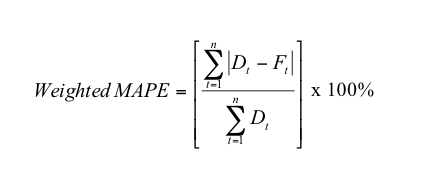
The disadvantage of using MAPE is that stock keeping units (SKUs) with low-volume demand can actually skew this metric. This can be overcome by using the weighted MAPE instead. The formula for the weighted MAPE shown in Figure 5 gives more weight to SKUs with higher demand. Note that this metric can be further customized by weighting the MAPE values by the dollar value of the SKU.

Figure 5
A weighted MAPE formula

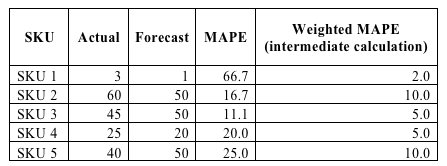
Table 1
An example of a MAPE and weighted MAPE comparison
MAPE for the above data is 27.9 and weighted MAPE is 18.7 across SKUs. In most organizations in which forecast accuracy is tied to performance of the planners, this difference becomes very important.
In addition to bias and accuracy, there are measures of forecast volatility using metrics such as weighted coefficient of variance (WCOV). However, these measures are rarely used in practice. According to the American Production and Inventory Control Society and Institute of Business Forecasting and Planning (APICS& IBF) 2012 “Sales & Operations Planning Report,” MFE and MAPE are the most commonly used metrics across industries.
When deciding which metrics to use, assess whether the metrics used are intuitive, easy to understand, and explainable to a wide audience. This is especially true if forecast accuracy is used as a metric to determine performance incentives for the supply chain or sales functions. Forecast accuracy metrics should be considered during the design of the demand planning process/ system to potentially reduce revisiting the demand-planning design.
Level of Aggregation
Forecasts can be more accurate in the aggregate. However, they may be correspondingly less useful for upstream supply chain planning. Consider these criteria when deciding at what aggregation levels to measure forecast accuracy:
- The appropriate level of aggregation is the one in which major business decisions on resource allocation, revenue generation, and inventory investment are made. For example, for planning of long-term capacity, it might make sense to aggregate forecast or history at the product line manufacturing plant level for the purposes of forecast accuracy. (Depending on the m:n relationship of the product or distribution center to the product or manufacturing plant, this may be a relatively simple aggregation or require complex sourcing rules.) However, for near-term inventory deployment decisions, forecast accuracy at a detailed product or distribution center is most relevant.
- Track accuracy across like items. For example, if you have different service levels for fast-moving items versus slow-moving items, then you may want to be able to calculate metrics at that level. You may also want to track accuracy by the product life cycle state — new products versus mature products.
- Track accuracy by forecast ownership — such as product family or sales regions
- Track accuracy at multiple levels — Users should be able to drill down to detailed levels to identify root cause of forecast accuracy issues.
- Maintain consistency over time for aggregation levels when reporting.
Forecast Types
In a typical collaborative sales and operations (S&OP) process, there may be several forecast inputs or outputs captured (including statistical forecasts, sales forecasts, marketing forecasts, and consensus forecasts). At the very least, measure accuracy for the forecast used by operations to build or procure the product — typically the consensus forecast.
Measuring accuracy against multiple forecasts provides greater insight into potential areas for improvement. For example, if your statistical forecast is more accurate in the long term, but your sales forecast is more accurate in the short term, perhaps you can combine these two to come up with a final forecast that is a combination of these two separate forecasts.
Measuring accuracy at each step of the demand planning process allows you to perform a forecast value-added (FVA) analysis. An FVA is the change in a forecast performance metric (such as MAPE) that can be attributed to a particular step of the demand planning process.
An FVA analysis is important because it helps you identify waste in your forecasting process. By identifying and eliminating the activities that are not making the forecast better, you can simplify your process and potentially improve the forecast accuracy. For example, for stable demand products, if you see that the FVA by the sales team (by means of an override) is negative, it might make sense to just use the baseline statistical forecast.
Lag (Offset)
Forecasts may be more accurate in the near term. That’s because you have better information as you get closer to the current period. However, accurate forecasts in the very near term are not much use to the business if the organization cannot act upon that forecast.
The lag or offset period defines the number of periods prior to an actual period for which a forecast is measured against the given period’s actuals. For example, if you measure the accuracy of the forecast for the month of August and the forecast was generated in May, you are measuring accuracy with a three-month lag.
Lag or offset should align with the organization’s planning horizons. Even within the same organization, there are likely to be multiple planning horizons based on business or product line. Planning horizons could also be different for different purposes — e.g., long-term capacity planning versus short-range inventory deployment.
Typically, industries that use make-to-stock manufacturing strategies use shorter lag or offsets for calculating forecast accuracy compared with industries that use make-to-order manufacturing strategies. Your forecast accuracy lag could also be influenced by transportation times if you have a global distribution network.
Buckets or Horizons
Typically, you want to measure accuracy in the same period buckets used to forecast. If demand patterns follow a high demand in the last month of a quarter, it may be more appropriate to use quarterly buckets. (However, this might promote continued bad behavior.)
The forecast accuracy horizon is the period of time over which to average accuracy metrics for reporting. Typically, this should be greater than the planning horizon, but short enough to be meaningful based on seasonality and business cycles. The horizons for bias calculations could be different compared with those for forecast accuracy calculations.
The number of archival forecast periods required in SAP Enterprise BW is based on a combination of lag (offset) + forecast accuracy horizon. For example, if you want to measure a three-month lag forecast over a horizon of 12 months, you need at least 15 months of forecast or actuals to make the calculation meaningful.
Units versus Dollars
Forecast accuracy can be measured in both units as well as dollars. High accuracy at the unit level with poor accuracy at the dollar level could indicate incorrect assumptions about the selling price.
Accuracy measures, such as weighted MAPE, provide greater influence to items that constitute a greater portion of the sales volume. Higher dollar, but low-unit volume items contribute much more to a measurement in dollars. Conversely, high-unit volume, low- dollar items factor in more prominently by using a unit-based forecast.
Industries that make low-volume, high-dollar products (e.g., industrial machinery) typically focus on unit measures because they have an S&OP process focused on capacity. Conversely, industries that make high-volume, low-dollar products (e.g., consumer packaged goods) tend to additionally use dollar metrics.
Representative Architecture Using APO DP and SAP BW
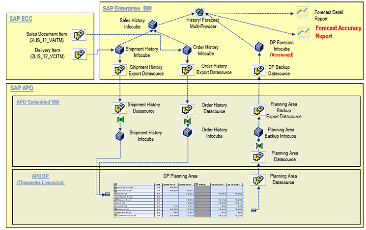
Figure 6 shows a representative technical architecture for measuring forecast accuracy. Although SAP provides standard BW structures (such as DataSources and InfoCubes) for several data objects such as sales history and forecasts, these usually need to be enhanced or custom built to meet enterprise specific requirements.

Figure 6
Representative architecture for forecast accuracy measurement
Key highlights include:
- Sales history (shipments or orders) is extracted from the SAP ECC system using standard available data sources. This history is updated into InfoCubes in Enterprise BW. These InfoCubes can be used for general sales reporting, as a repository or staging area for data to be sent to APO BW as well as the basis for forecast accuracy reporting.
- Sales history is transferred into InfoCubes in APO BW and then loaded into the DP planning area. History can be used for statistical forecasting or for planner reference.
- Multiple forecasts (such as statistical, sales, marketing, or consensus) are generated in APO DP.
- On a periodic basis, the data in the planning area is backed up into InfoCubes in APO BW (with overwrite of existing planning data).
- Periodically, forecasts (not history) from APO BW are copied into InfoCubes in Enterprise BW with versioning (without overwrite of existing data).
- A multi-provider in Enterprise BW is used to combine sales history and forecast data. BW queries based on this multi-provider are used for forecast accuracy reporting.
- BW queries are used to define two types of reporting outputs: operational drill-down type reports for in-depth analysis by demand planners as well as high level dashboards for senior management.
Tips for Implementation
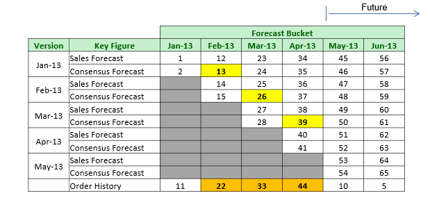
For performance reasons, it is useful to pre-calculate lag values and store them in Enterprise BW while versioning (storing data) instead of calculating it as part of the BW query. Table 2 shows an example of how lag values are calculated and stored in Enterprise BW. The Forecast Bucket identifies the calendar month the forecast is for. The ‘version’ identifies the calendar month when the forecast from APO BW was versioned into Enterprise BW. The lag is calculated as the number of months between the forecast version and the forecast bucket.

Table 2
An example of forecast capture with various lag values
Tip
In the BW query, set the exception aggregation parameter for calculated key figures (forecast accuracy metrics) to a value ‘Average’. This allows the report to aggregate across characteristics such as material, plant, or customer but not across calendar months.
Let’s take an example of how lag is considered in the accuracy calculation. Figure 7 shows representative data in the enterprise BW system.

Figure 7
Lag calculation
- Lag: One month
- Horizon: Three months
- Forecast type: Consensus forecast
The BW query identifies the history and forecast values (Figure 8).

Figure 8
Lag calculation – data used for forecast accuracy metric
The above example shows that to correctly calculate forecast accuracy with lag, the system needs to determine the forecast quantity for each bucket across the horizon from different versions. The query can be simplified by pre-calculating and storing the lag value at the time of versioning and using the lag value as a filter in the BW query.
Forecast accuracy metrics help drive operational excellence across the supply chain as well as enabling good S&OP processes. An increase in forecast accuracy can have a significant impact on the financial top line and bottom line of an enterprise. We have summarized the leading practices for how a company could use select metrics for accuracy calculations. We also have explained how such metrics can be implemented in an SAP environment that has APO DP and SAP BW as part of its landscape.
This article contains general information only, and none of the member firms of Deloitte Touche Tohmatsu Limited, its member firms, or their related entities (collective, the “Deloitte Network”) is, by means of this publication, rendering professional advice or services. Before making any decision or taking any action that may affect your business, you should consult a qualified professional adviser. No entity in the Deloitte Network shall be responsible for any loss whatsoever sustained by any person who relies on this publication.
As used in this document, "Deloitte" means Deloitte Consulting LLP, a subsidiary of Deloitte LLP. Please see www.deloitte.com/us/about for a detailed description of the legal structure of Deloitte LLP and its subsidiaries. Certain services may not be available to attest clients under the rules and regulations of public accounting.
Copyright © 2014 Deloitte Development LLC. All rights reserved.
Rishi Menon
Rishi Menon is a specialist master at Deloitte Consulting LLP, with more than 17 years of supply chain and enterprise application consulting experience. He specializes in supply chain planning and order fulfillment. He is SAP SCM, APICS (CPIM, CSCP & CIRM) and PMI (PMP) certified.
You may contact the author at rimenon@deloitte.com.
If you have comments about this article or publication, or would like to submit an article idea, please contact the editor.
Satish Vadlamani
Satish Vadlamani (Ph.D., PMP) is a senior independent SAP Advanced Planning and Optimization (APO) consultant and president of SAPsquad Inc. He has more than 15 years of SCM consulting experience in various industries. He specializes in SAP SCM consulting and service offerings.
If you have comments about this article or publication, or would like to submit an article idea, please contact the editor.
