Forecasting in SAP ERP is one of the lesser-used planning tools that can help predict your procurement and production requirements effectively. While advanced planning tools such as SAP Advanced Planning & Optimization (APO) can certainly bring greater business process optimization to the company, using this forecasting tool helps a company get a better return on its SAP ERP system.
Key Concept
A forecast is a prediction of future requirements based on the past consumption trend in a given period of time. These consumptions can be, for example, a material withdrawal against the production or process order or even cost center. Forecasting in SAP ERP enables you to plan any type of material, be it a raw material, a consumable, or a semi-finished or finished good. Different forecasting models, such as constant and moving averages, help you to accurately predict demand for a product based on historical consumption values.
To demonstrate the forecasting functionality in an SAP ERP system, I enter a few historical figures, select the correct forecasting model, and then run a forecast to come up with a future prediction for quantities of materials. I also point out the specific location in the material master that automatically records past consumption. You can use it to evaluate the consumption pattern and to see how it differs from your forecasting and planning results.
Forecasting is not only available for use as a stand-alone planning tool. In fact, you can also use it to plan those materials that eventually form a part of material requirements planning (MRP). Some MRP types available in the system require you to run the forecasting before you run MRP. Forecasting finds greater relevance in SAP ERP components such as materials management (MM), production planning (PP), and sales and distribution (SD). To begin using forecasting to your business advantage, you need to ensure that the forecasting view in the material master is activated.
Forecasting in the SAP ERP system makes use of both planned and unplanned historical consumption data. You can choose from several preconfigured forecasting models including constant, moving average, and seasonal average, and can run forecasting on any material type, be it a finished good or a consumable item. Smoothing factors such as alpha, beta, or gamma, smooth the forecast values of materials. The forecast profile enables you to set up default values that you can use to save time and effort in forecasting and provides the flexibility to make any last minutes changes needed.
Warning
Although an automatic model selection is available to help you with the correct forecast model selection, it comes with a warning from SAP: SAP does not recommend making use of an automatic model selection for forecasting, as it can eventually end up incorporating one of the several forecast models (such as constant, moving average, or seasonal) available in the material master. The SAP-recommended model may not be in line with your business scenario and thus may not meet your planning needs effectively. It is a prudent and a practical approach to revisit your forecasting model in the material master occasionally to ensure that the correct forecasting model is in place.
Whenever you create a new material in the system, the system automatically incorporates the Consumption tab in the Additional Data of the material master. While each withdrawal or consumption updates the information in the system, you can also manually enter past consumption figures of a material to help drive and facilitate forecasting.
A detailed analysis of the consumption figures provides a pattern or valuable information on the consumption pattern, that is, a constant consumption, a moving average, a seasonal, or seasonal trend model.
Forecasting View in Material Master
You can enter the forecast parameters in the forecasting view of material master using transaction MM02. Figure 1 is the material master change screen. Select the Forecasting view for material 100-110 and press Enter. The system brings up Figure 2, which is the organizational data view of the material master.

Figure 1
Forecasting view selection for material master
Figure 2 is the organizational levels view. Enter Plant 3000 and press Enter. The system navigates to the screen shown in Figure 3. Since consumption of a material is stored at the plant level, you have to specify the plant in addition to the material master in order to run the forecast.

Figure 2
Organizational levels (Plant) selection for material master
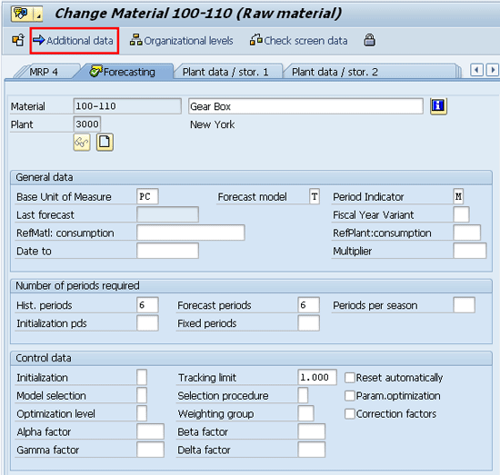
Figure 3 is the Forecasting view of material master 100-110 for plant 3000. Before I discuss the forecasting parameters of Figure 3 in detail, let’s first explore where the system stores the consumption data or where you can manually enter it if there isn’t any historical consumption data.

Figure 3
Forecasting view selection for material master
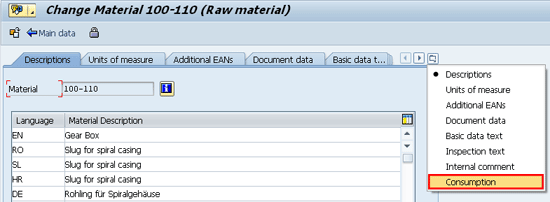
Click the Additional data button in Figure 3, and the system navigates to the screen shown in Figure 4. This screen contains several tabs of additional data of a material master. Here, I select the Consumption tab, and the system brings up the screen shown in Figure 5.

Figure 4
Additional data view of material master with consumption option

Figure 5
Unplanned consumption of the material master-plant combination
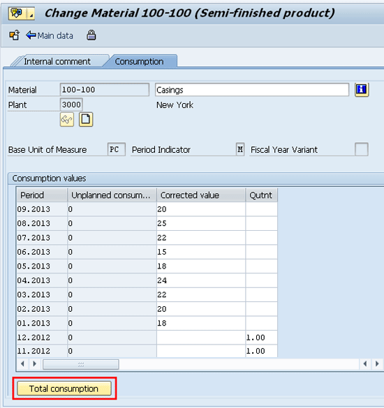
Figure 5 is the consumption tab of the material 100-110 and plant 3000 combination. As noted previously, that consumption data (or the tab) is only available when you select the material-plant combination. In this figure, the system brings up both planned and unplanned consumption data. Planned consumption data is, for example, the actual goods issuance of a material against a production order. However, if there was additional issuance of material against a cost center, the system records it as unplanned consumption.
Here, I manually enter the monthly consumption data for nine months. If needed, you can always manually enter the consumption data. This option is useful when you are implementing an SAP ERP system for the first time and you’d like to record historical consumption values of a material to be able to immediately start taking advantage of the forecasting tool that the system offers. Click the Total consumption button in Figure 5, which takes you to the screen shown in Figure 6.

Figure 6
Total consumption of material (planned and unplanned)
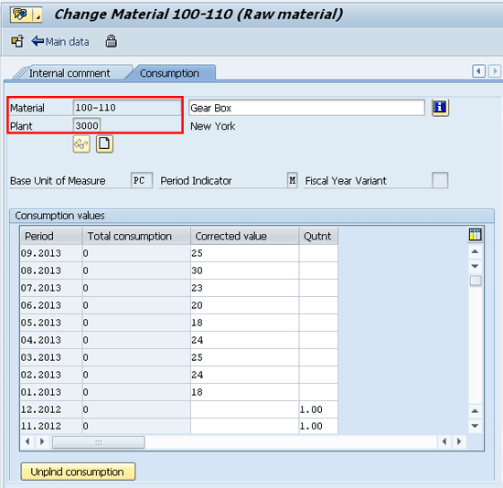
Figure 6 provides you an option to record both planned and unplanned consumption by means of entering total consumption for a material-plant combination. If you make use of consumption-based planning, such as manual or automatic reorder point planning, then the system automatically updates the total consumption data based on the withdrawal or consumption. Here, I manually enter the total consumption figures to make it more than the unplanned consumption figures. Click the back icon (not shown) in Figure 6 and the system navigates to Figure 7, which again is the forecasting view of the material.

Figure 7
Forecasting view selection for material master
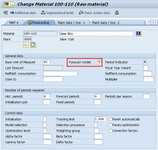
Figure 7 is the upper-section of the Forecasting view of the material master. The system provides you the option to select the relevant forecast model. It also allows you to select a period indicator, which means you can split your forecasting values not just by monthly figures but also weekly or even daily figures. Furthermore, if you want to use the forecasting parameter’s results on a reference material to forecast for the current material, then you can assign the reference material and it’s reference plant in the ReflMat:Consumption field together.
You can also control how the forecast values of the reference material correspondingly increase or decrease the forecast results by entering a multiplier. For example, if you want to use only 80 percent of the reference material’s consumption to execute a forecast for your current material, then you can enter 0.8 in the multiplier field.
You can define the number of historical periods that the system should consider in forecasting, as well as the number of forecast periods to predict after running the forecast. In my example, I assign 6 to both historical periods and forecast periods. The system reads the last six historical figures and comes up with six new forecast figures after running the forecast.
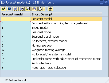
Place the cursor in the Forecast model field and press F4 (or click on the dropdown) in Figure 7. The system opens a popup screen to select from one of many forecast models (Figure 8).
Note
When you run the forecast for a material-plant combination (transaction MP30) or for the entire plant (transaction MP38,) the system makes use of information from the material master. It offers no option to make changes in the forecast parameters. You can navigate to the Forecast menu in SAP via Logistics > Production > Production Planning > Materials Forecast.
Figure 8 provides a list of SAP-delivered forecast models that you can immediately start using. In my example, I select the forecast model T (Trend model) shown in Figure 7. Scroll down in the screen in Figure 7 to get to the screen in Figure 9.

Figure 8
Forecast models

Figure 9
Executing forecast option in the material master
Figure 9 is the remaining screen of the Forecasting view. Here, depending on the model selected, the system makes use of smoothing factors, which improve the accuracy of forecast figures by harmonizing, or smoothing, sudden peaks or drops in the figures.
- Alpha factor smoothes the basic value.
- Beta factor smoothes the trend value.
- Gamma factor smoothes the seasonal index.
Now you execute the forecast by clicking the Execute forecast button in Figure 9. The system brings up the popup shown in Figure 10.
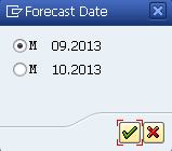
In Figure 10, you can select if you want the system to start the forecast from the current month or from the next month. In my example, I chose 09.2013 (September, 2013) as the current month and clicked the continue icon. This time the system brings another pop-up, as shown in Figure 11.

Figure 10
Forecast period

Figure 11
Forecast model selection
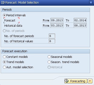
Figure 11 provides you an option to change the forecast model if there’s any such last-minute need for it. I still select the Trend model’s radio button and click the Forecasting button. This brings up another screen shown in Figure 12.

Figure 12
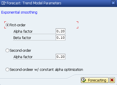
Forecast trend model parameters
Figure 12 Forecast trend model parameters
Figure 12 shows that, since I am using Trend models, the system prompts me to make use of Alpha and Beta factors for smoothing. You can either use the smoothing factors that the system proposes or you can overwrite them with your own desired values. Click the Forecasting button in Figure 12 and the system brings up the forecast results, as shown in Figure 13.

Figure 13
Forecast results
Figure 13 is the system-generated forecast values for the next six periods (months). Notice that it has considered total consumption figures (and not just planned or unplanned consumption) to come up with the forecast values.
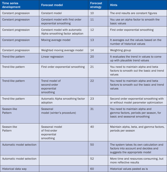
Table 1 shows the logical link between various forecast models, such as trends or seasonal trends, and the use of smoothing factors. For each forecast strategy (or model) selection, you will have to give details of the parameters, such as Alpha factor, Beta factor, or Gamma factor. This is highlighted in the Hints column of the table. For example, if the demand of a product is generally constant throughout the year, then you should select the constant model. Similarly, if you wish to maintain an average quantity of material in the warehouse, then you should use the moving average model. In moving average, the system adds up the total quantity of the material from historical figures and then divides this total quantity with the period under consideration to arrive at an average number.

Table 1
Forecast models and forecast strategies
While my example shows you how you can use the forecasting tool for a material, you can also execute a forecast in:
- Sales and Operations Planning for a material or product group
- Demand Management as in Planned Independent Requirements (PIR)
- Flexible Planning

Jawad Akhtar
Jawad Akhtar earned his chemical engineering degree from Missouri University of Science and Technology. He has 17 years of professional experience, of which nine years are in SAP. He has completed eight end-to-end SAP project implementation lifecycles in the areas of PP, QM, MM, PM, and DMS in the steel, automobile, chemical, fertilizer, FMCG, and building products industries. He also has worked as an SAP integration manager and an SAP project manager. He has been proactively involved in a business development and solution architect role for seven years. He is the author of Production Planning and Control with SAP ERP, it's filled with in-depth infomation on discrete, process, and repetitive manufacturing types. His profile on LinkedIn is at https://pk.linkedin.com/in/jawadakhtar. You may follow Jawad on Twitter @jawadahl. Currently, he is associated with AbacusConsulting as Head of SAP Delivery.
You may contact the author at jawad.akhtar@live.com.
If you have comments about this article or publication, or would like to submit an article idea, please contact the editor.


