Consider a scenario in which company AZBY is a manufacturer of pumps. During the manufacturing of pumps, company AZBY also produces other co-products, such as two different types of sheet metals as well as remnants of sheet metals. Therefore, for this scenario, pump (Material ID: T-COP) is the primary co-product (i.e., the main finished product). The remaining three co-products are sheet metal ST37 (T-COP1), sheet metal ST38 (T-COP2), and sheet metal remnants (T-COP3), respectively. The quantity produced for the three co-products is 0.05 M², 0.03 M², and 0.10 M², respectively, for the production of one pump. The costs to manufacture a pump and associated three co-products are categorized in three distinct categories: material costs, production costs, and miscellaneous costs. The ratio of cost allocation across all co-products is different for each cost category. I explain the following product costing steps that company AZBY needs to complete for joint production processes during the manufacturing of its pumps:

1. Set up the material master for the T-COP with the allocation and source structure
2. Set up a bill of material (BOM) for the T-COP
3. Calculate the standard cost for the T-COP
4. Complete the production order and cost object controlling processes for joint production

The case study for this article includes four co-products; namely, T-COP, T-COP1, T-COP2, and T-COP3. T-COP is the primary co-product. First, I explain the material master setup of T-COP, the significance of allocation and source structure assigned to T-COP material master data, and the configuration of the source structure. If the source structure is assigned to the material master, you can define a different ratio of cost allocation for each cost category. A source structure enables you to classify the costs in different categories based on the origin of the cost. If a source structure is assigned to an apportionment structure in the material master, you can define the ratio of cost apportionment across co-products for the cost categories configured for the source structure. If no source structure is assigned to the apportionment structure in the material master, the cost apportionment ratios cannot be defined for different cost categories, and only one ratio applies to the total cost. Therefore, without a source structure, the cost apportionment ratio can be defined for total cost only, and different ratios for different cost categories cannot be defined.

Step 1. Set Up the Material Master for the T-COP with the Allocation and Source Structure

To complete this step, execute transaction code MM03 or follow menu path Logistics > Production > Master Data > Material Master > Display > Display – Current. In the screen that appears (Figure 1), enter T-COP in the Material field, enter 1000 in the Plant field, and click the Costing1 tab.

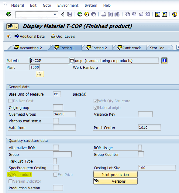
Figure 1

Costing1 view of the primary co-product material master

You also need to select the Co-product check box (highlighted in yellow in Figure 1) in the Quantity structure data section of the Costing1 tab of the material master in order for the SAP system to recognize that this material is a co-product.  This check box needs to be set up for all the co-products (in this case study all four products (i.e., T-COP, T-COP1, T-COP2, and T-COP3).

In addition to selecting the Co-product check box, you need to set up in the material master data of the T-COP percentage apportionments of the estimated and actual costs for each of the four co-products For this example, T-COP has three secondary co-products. In Figure 1, click the Joint production button next to the Co-Product check box to review the allocation of the estimated (standard) cost as well as actual cost among the primary co-product T-COP and its three co-products.  After you click the Joint production button, the system displays a screen that shows the allocation structure 0001 defined for T-COP cost allocation (Figure 2).

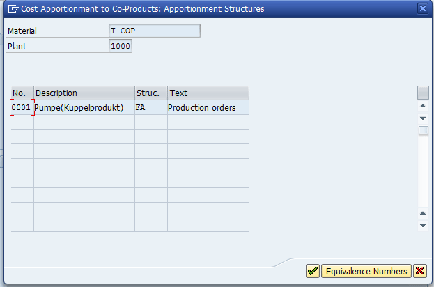
Figure 2

Allocation structure of the material T-COP and co-products

In Figure 2, you can see four columns for the material T-COP. The first column (No.) specifies the apportionment structure, and the third column (Struc.) specifies the source structure. The apportionment structure contains the equivalence numbers that determine the proportion of costs to be distributed among each co-product.

In addition, the source structure helps if the cost distribution proportion differs based on the origin of the cost (cost category). The source structure allows setting up different equivalence numbers for different cost categories (i.e., costs of different origins). In Figure 2, for my example, you assign an allocation structure of 0001 (first column) and a source structure of FA (third column) to the material master of T-COP. Click the green check mark after entering your data.

Before I explain the material master setup further for T-COP1 and how the combination of allocation structure 0001 and source structure FA help set up cost allocation ratios across all four co-products, I explain the configuration of source structure FA.

To configure source structure FA, follow IMG menu path Product Cost Controlling > Cost Object Controlling > Period-End Processing > Settlement > Create Settlement Structure. In the screen that appears (Figure 3), select the source structure FA, expand the Source structures folder, and then double-click the Assignments folder.

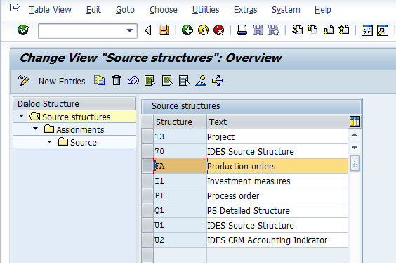
Figure 3

Configuration of source structure FA

This action opens a screen that displays the assignments of various cost categories to the source structure FA (Figure 4). The three cost center categories assigned to source structure FA are Material Costs, Production Costs, and Miscellaneous Costs. Because source structure FA is assigned to the apportionment structure of material T-COP, the three cost categories are available for apportionment for material T-COP and its co-products.

Figure 4

Assignment of various cost categories to source structure FA

Select the Material costs category in Figure 4 and then double-click the Source folder. This action displays the screen shown in Figure 5. In Figure 5, Cost Element Group CO-PC-MAT is assigned to material costs. I assume that readers are aware of cost element groups and therefore, explanation of cost elements assigned to cost element group is not given here to avoid digression from the subject of the article.

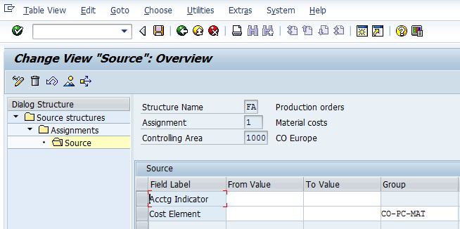
Figure 5

Cost element assignment to the source structure cost categories

The source structure FA includes three distinct cost categories: material costs, production costs, and miscellaneous cost. In Figure 2 of the T-COP material master, the source structure helps to define a different equivalence number (i.e., a different ratio of cost allocation for each category). To display the apportionment of the costs pertaining to different origins (i.e., material costs, production costs, or miscellaneous costs across all four co-products), follow the instructions to access Figures 1 and 2 and click the Equivalence Numbers button in Figure 2. This action opens the screen shown in Figure 6. (Note: Figure 6 shows equivalence numbers for material costs and production costs. To see, equivalence numbers for miscellaneous costs, you need to scroll further down in Figure 6 (the miscellaneous costs are not shown in Figure 6). Table 1 shows the details of equivalence numbers for miscellaneous costs.)

Figure 6

Cost apportionment for T-COP and its co-products

What does the equivalence number do? For material costs, equivalence numbers are totaling to 100 (90+2+5+3 =100). So, if material costs incurred to produce T-COP are $100, costs apportioned to T-COP, T-COP1, T-COP2, and T-COP3 are $90, $2, $5, and $3, respectively.  Table 1 shows the overall allocation of costs for all three cost categories.

Source structure FA helps to define different equivalence by each cost category. If source structure FA is not assigned to apportionment structure 0001 in Figure 2, only overall equivalence among all co-products can be defined (i.e., the allocation of costs by cost category would not have been feasible without source structure assignment).

Step 2. Set Up a BOM for the T-COP

Now I explain the BOM setup required for the joint production scenario. Note that the BOM needs to be created for the primary co-product only. Therefore, for my example, the BOM needs to be defined for T-COP only.

Two settings are required for the BOM of the main product:

• Specify negative quantity of co-products
• The Co-product check box is set for co-products items

To display the BOM, execute transaction code CS03 or follow menu path Logistics > Production > Master Data > Bills of Material > Bill of Material > Material BOM >Display. The screen that appears (Figure 7) shows the BOM of main product T-COP for which co-products T-COP1, T-COP2, and T-COP3 are specified as components of the T-COP and negative quantity is entered for the co-product items (item numbers 71,72, and 73).

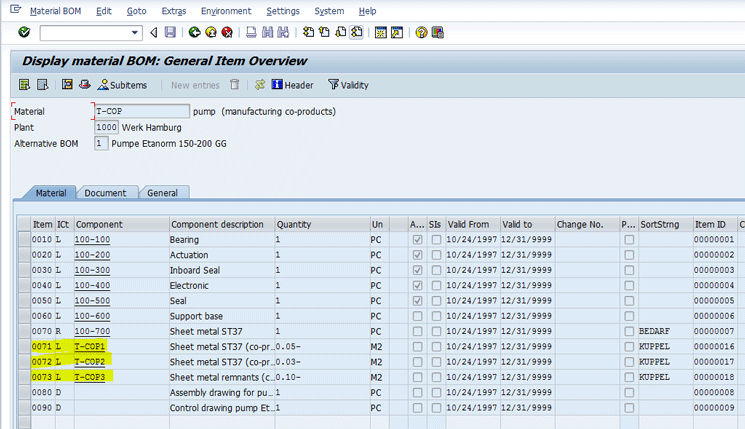
Figure 7

BOM setup for T-COP1

Select item 71 and then double-click the quantity cell for that item. This action opens a screen that displays the details of that BOM item (Figure 8). As explained, the Co-product check box is selected for the item 0071.

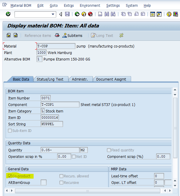
Figure 8

BOM item for the co-product T-COP1

Step 3. Calculate the Standard Cost for the T-COP

To explain how the material master and BOM setup for joint production affect the standard cost calculation, execute transaction code CK11n to analyze the standard cost calculated by the system for the primary co-product T-COP.  I assume that readers are well acquainted with the standard cost calculation transaction (edit costing run [transaction code CK40n] or cost estimate with quantity structure [transaction code CK11n]). Therefore, I focus on the analysis of the end result after executing transaction code CK11n (i.e., T-COP and co-product standard cost calculated by the system).

To create a material cost estimate with quantity structure for the T-COP, execute transaction code CK11n. In the screen that appears (Figure 9), click the icon at the end of the Material field and select T-COP from the list of options. Enter a value (e.g., 1000) in the Plant field and populate the Costing Variant, Costing Version, and Transfer Control fields as shown in Figure 9.  

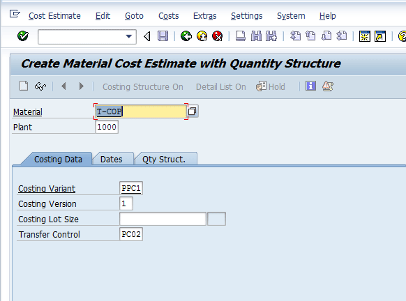
Figure 9

Create a material cost estimate with quantity structure for T-COP material

Now click the Dates tab (Figure 10). Click the icon at the end of the Costing Data From field and select a date from the drop-down list of options. Enter dates in the Costing Date To, Qty Structure Date, and Valuation Date fields. Press the Enter key after you make your selections.

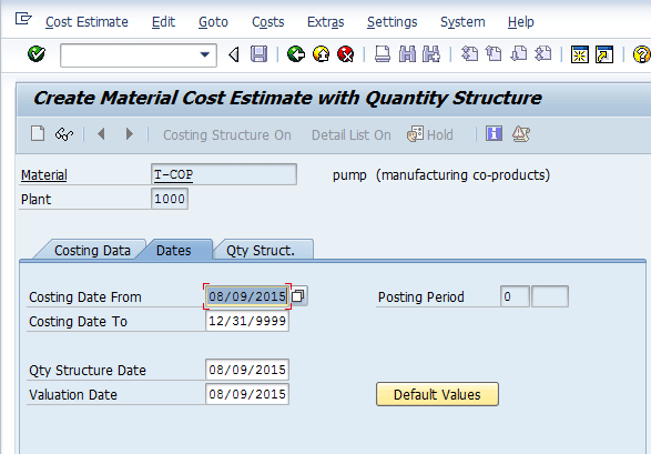
Figure 10

Enter dates for the material cost estimate with quantity structure for material T-COP

The next screen (Figure 11) displays the material cost estimate with quantity structure for material T-COP that you just created.

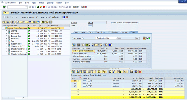
Figure 11

Standard cost for T-COP

Note that the standard cost calculated for T-COP is $4,576,654.62 for the quantity of 100 pieces as the costing lot size set up for T-COP is 100 pieces. The right bottom section in Figure 11 shows the cost by different item categories (the I… column highlighted). The costs by three item categories A, E, and M are - $569,145.42, $1,091,307.24, and $4,054,492.80, respectively.

Item categories A, E, and M represent co-products, activity (machine hour or labor hours, etc.), and raw material or semifinished products, respectively. In fact, the total cost for producing 100 pieces of T-COP1 is the total of item categories E and M ($5,145,800.04).

This total is distributed across all the co-products based on the equivalence numbers set up (Figure 6). Therefore, the cost allocated to T-COP1, T-COP2, and T-COP3 is subtracted from total costs to derive standard cost for the primary co-product T-COP.  The cost for item category A is the total cost allocated to co-products T-COP1, 2, and 3 and is negative as it is subtracted from the total cost. Table 2 shows the standard cost allocation across all the co-products using equivalence numbers set up for allocation structure for cost category.

Complete the Production Order and Cost Object Controlling Processes for Joint Production

In joint production, a production order is created for the primary product. The system recognizes from the material master settings that the primary product is a co-product.  For my example, T-COP is the primary product. To display the production order 60006249 that you created earlier for 1 quantity of T-COP, execute transaction code CO03 and follow menu path Logistics > Production > Shop Floor Control > Display Order. The screen that appears (Figure 12) displays the production order.

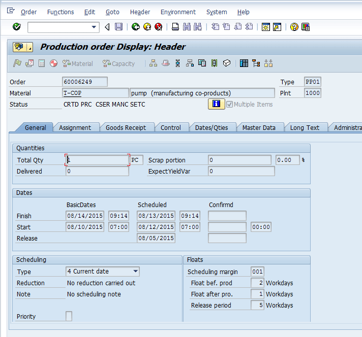
Figure 12

Production order for production of primary co-product T-COP

When the production order is created for the primary products, the system creates an order item for each co-product specified in the material master of the primary product. To review order items for order 60006249, click the Goto button in Figure 12 and follow menu path Overview > Object Overview. The next screen (Figure 13) shows the overview of the production order 60006249, which has four order items. The first order item is for the primary co-product T-COP. The remaining three order items are created for the remaining co-products: T-COP1, T-COP2, and T-COP3.

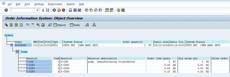
Figure 13

Order items for the production order 60006249

The planned quantity for production order 60006249 comes from the BOM of the primary product T-COP. The negative quantity of co-products T-COP1, T-COP2, and T-COP3 in the BOM implies that 0.05 M², 0.03 M², and 0.10 M² are manufactured  as shown in Figure 13 while to manufacture one piece of T-COP.

The system defaults settlement rules based on the equivalence number set up in the material master of the primary co-product T-COP. The equivalence numbers for the material T-COP are shown in Figure 6 and Table 1. To review settlement rules, go to Header Menu > Settlement Rule within Display Order transaction. The settlement rule for production order 60006249 is shown in Figure 14.

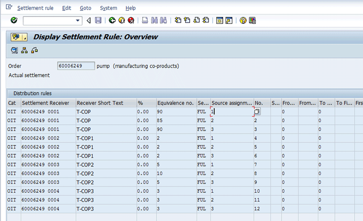
Figure 14

Settlement rule for the production order 60006249

Figure 15 shows the description of numbers appearing in the Source assignm… (source assignment) column in Figure 14.

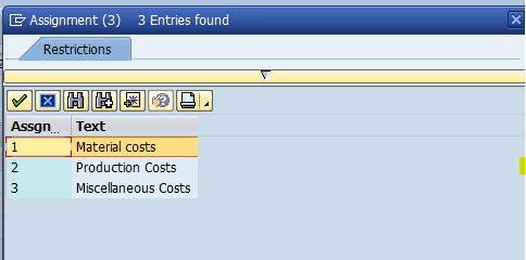
Figure 15

Source assignment descriptions

Setting up the material master with co-product indicator and other requisite settings as explained in earlier sections of master data helps in the following ways.

Because a production order is created with order items for each co-product, the system proposes the entering of the actual production of each co-product while entering a good receipt for the production order. To complete this process, execute transaction code MIGO and follow menu path Materials Management > Inventory Management > Goods Movement. Figure 16 shows the goods receipt proposal for all the four co-products as the system has created four order lines for production order 60006249.

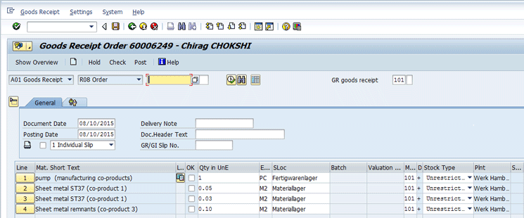
Figure 16

Goods receipt proposal for the production order 60006249

The quantity proposal for each co-product defaults from the BOM of the primary co-product.

Unlike other production orders with multiple order items, the production order for the co-products collects all the costs on the header. However, the costs are not distributed to the order items until the transaction preliminary settlement for co-products is executed. For my example, execute the variance analysis for the production order 60006249 prior to and after execution of preliminary settlement of the co-products.

To review the status of the order, execute transaction code CO03 or follow menu path Logistics > Production > Shop Floor Control > Display Order.  Because the order is fully delivered for all the co-products’ order items, the status of order 60006249 changes to DLV (fully delivered) as shown in Status field of Figure 17.

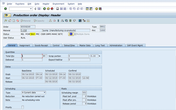
Figure 17

Status of order changes to DLV

Now, because the status of order 60006249 is DLV, variance calculation can be executed for this order. First, execute the variance calculation before executing preliminary settlement. To execute the variance calculation use transaction code KKS2 for individual order or follow menu path Controlling > Product Cost Controlling > Cost Object Controlling > Product Cost by Order > Period End Closing > Variances > Individual Processing. In the screen that appears (Figure 18) enter 60006249 in the Order field. In the Parameters section, enter 8 in the Period field, enter 2015 in the Fiscal Year field, and select the Selected Target Cost Vsns radio button. In the Processing options section, select the Test Run check box to execute variance analysis in test mode. You also select the Detail list check box. After you enter all your data, click the execute icon.

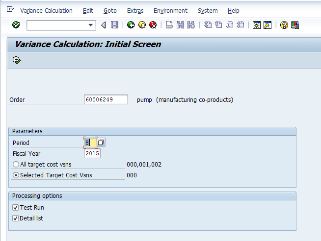
Figure 18

Variance calculation for the production order 60006249

The next screen (Figure 19) displays the output of the variance calculation report output. Note that there is no actual cost accumulated on any of the production order line items as the amounts listed in the Actual Costs column are all 0.00. Because the goods issues and confirmations are posted on order 60006249, you expect actual costs to appear for order line items. However, because preliminary settlement is not yet executed, the actual costs captured on the order header are not distributed to order items. Therefore, variance calculation is inaccurate if it is executed prior to preliminary settlement.

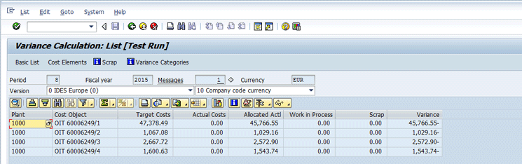
Figure 19

A variance analysis report prior to execution of preliminary settlement

Now, execute the preliminary settlement in test mode. Use transaction code CO8B for individual order and follow menu path Controlling > Product Cost Controlling > Cost Object Controlling > Product Cost by Order > Period End Closing > Preliminary Settlement for Co-Products, Rework > Individual Processing. In the screen that appears (Figure 20), enter 60006249 in the Order field and select the Test Run check box to execute preliminary settlement in test mode. In the Parameters section, enter 8 in the Settlement period field and 2015 in the Fiscal Year field. After you enter all your data, click the execute icon.

Figure 20

Preliminary settlement (test run execution) for production order 60006249

Using settlement rules as shown in Figure 14, the system distributes the total cost captured on the order header to the respective order items for each co-product produced with the production order. The result of preliminary settlement is shown in Figure 21.

Figure 21

Preliminary settlement of order costs to order items (each co-product)

Now click the Sender button (Figure 21) to view details of the cost elements and amounts posted to each cost element (Figure 22). The settlement rules shown in Figure 14 are the basis of preliminary settlement. These rules are derived from source structure assigned to material master of T-COP and then equivalence numbers are set up for each source structure category for each co-product. Table 3 lists the allocation of costs to each co-product.

Figure 22

Sender cost elements for header cost for production order 60006249

Cost elements 40000 and 890000 contain material costs for raw material and semifinished products. The remaining three cost elements belong to the production costs. The equivalence numbers are set up differently for material cost and production cost for T-COP and its co-products (as shown in Figures 3 and 14). Table 3 shows the overall distribution of the cost.

Now you execute the preliminary settlement in the update mode by deselecting the Test Run check box (Figure 20). After you run preliminary settlement in update mode (i.e., with the Test Run check box deselected), run the variance analysis again to compare results of variance calculation prior to and after preliminary settlement. The results of variance calculation after preliminary settlement is shown in Figure 23.

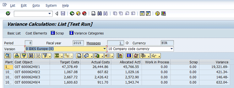
Figure 23

Variance analysis after preliminary settlement

Comparing variance calculation in Figures 19 and 23 indicates that the actual costs prior to preliminary settlement were zero for all co-products (Figure 19), whereas actual costs after preliminary settlement has non-zero actual cost (Figure 23) as allocated in Table 3 to all co-products. This allocation provides correct variances for each co-product. Therefore, preliminary settlement is a prerequisite for a joint production scenario for variance calculation and actual settlement.