Data Outliers Detection in SAP IBP Demand Forecasting

⇨ Understand the importance of data-preprocessing for demand forecasting.

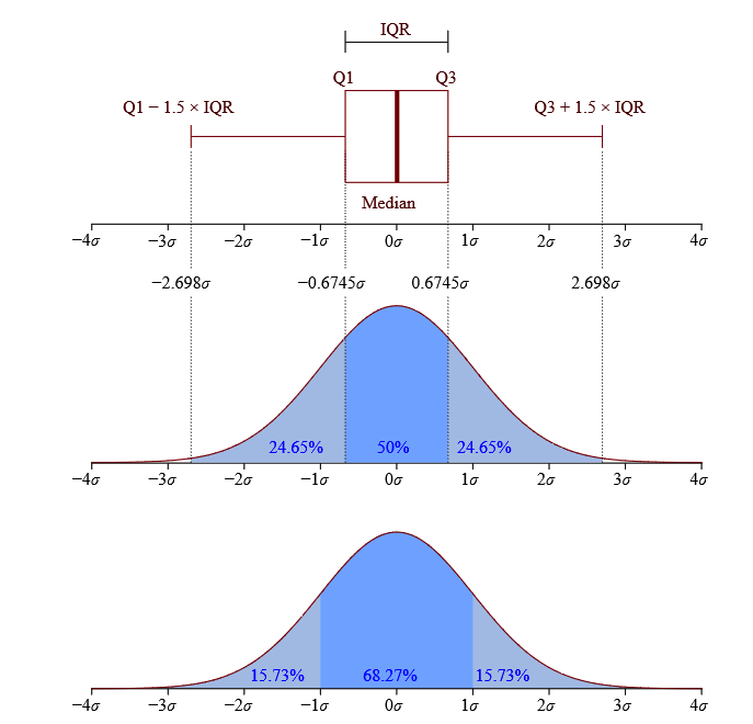
⇨ Learn about outliers in your input datasets and the features SAP IBP provides to address them.

⇨ Explore the details of the two methods SAP IBP makes available to its users for outlier detection.

In our recent research, Supply Chain Planning in The Cloud, SAPinsiders highlighted that demand forecasting remains a key challenge. Fortunately, best-of-breed supply chain tools today provide many features and functionalities, including a rich portfolio of algorithms, that can help bring more science and certainty into this exercise. However, as the popular saying of "Garbage-In-Garbage-Out (GIGO)" goes in the world of analytics, a significant portion of the quality of your forecasts is also dependent on data preprocessing. And best-of-breed solutions help users in this area as well. In this article, we will explore pre-processing steps and associated algorithms available to users in SAP IBP.