The sum of prices per product often is not an accurate measure of performance when comparing multiple vendors, materials, and prices. The weighted average method, however, adjusts the sums proportionately so that you can make an accurate judgment of vendor performance. While BW has no standard weighted average method of aggregation, you can model it in BEx Query Designer using calculated key figures.
Key Concept
The weighted average aggregation method makes quantities consistent at any drill-down level, without major changes to the back end, by using sums adjusted to reflect the proportionate prices of materials sold by different vendors.
In my work with clients, I have encountered several functional and technical issues involving product pricing. Aggregating the prices for comparison purposes is not as straightforward as simply adding the prices or taking the average of the prices because these figures are not consistent across drill-down levels. However, by weighting the averages, I can create a report that reflects the proportionate prices of each vendor across drill-down levels. This allows you to compare the purchasing price variance (PPV) to determine which vendor gives you the best value. I will show you how to use BEx Query Designer to model a weighted average aggregation method using calculated key figures.
Say you purchase three materials from two different vendors and you want to compare the performance of each vendor in July 2005 by using the purchasing performance report. Multiple vendors, materials, and prices are involved, so neither summation methods nor average methods present a consistent, accurate view of price reporting. Using the weighted average aggregation method lets you view price reporting in this situation and reflects all prices proportionately depending on the quantity sold in a given time frame.
Even if your reporting requirements on prices are not as complex as described in this article, you may find some of my tips and tricks useful. Purchasing is just one of the examples of the application of the weighted average aggregation method. You could apply the same methods described in this article to a Sales and Distribution (SD) report. For example, instead of vendors, you could use this method for customers. This functionality has proven to work with BW 3.x.
I’ll explain the theory behind the weighted average aggregation method and show you how it provides consistent reporting at all drill-down levels. Using my example of a purchase performance report, I’ll walk you through the thought process of setting up the necessary formulas, show you how to implement them in BW, and demonstrate how the weighted average aggregation method works for both drill-down by material and drill-down by vendor.
Build the Purchase Performance Report
To compare vendor performance, include the following key figures in your purchase performance report:
- PPV
- Material standard price
- Invoice actual price
- Actual quantity purchased
In addition, to make the comparison, you need to be able to drill down using the following characteristics:
Table 1 shows the transactional data of three materials (M) sold by two different vendors (V). Only the first four columns constitute the transactional data from the source system. Invoice actual price may also come directly from the source system, but it is better to calculate invoice actual price in the report using a calculated key figure that divides invoice value by invoice quantity. Not keeping the invoice actual price in the InfoCube allows better aggregation and unit of measure display, as I will show in my example.
| M1 |
V1 |
10 TO |
1400 EUR |
1400 EUR/TO |
1600 EUR/TO |
2000 EUR |
|
V2 |
2 TO |
4000 EUR |
2000 EUR/TO |
1600 EUR/TO |
-800 EUR |
| M2 |
V1 |
5 TO |
1500 EUR |
300 EUR/TO |
250 EUR/TO |
-250 EUR |
|
V2 |
20 TO |
5000 EUR |
250 EUR/TO |
250 EUR/TO |
0 EUR |
| M3 |
V1 |
5 TO |
3000 EUR |
600 EUR/TO |
650 EUR/TO |
250 EUR |
|
V2 |
25 TO |
15000 EUR |
600 EUR/TO |
650 EUR/TO |
1250 EUR |
|
| Table 1 |
Transactional data of three materials sold by two different vendors |
To aid my comparison in Table 1, I also added the material standard price and calculated the PPV, although these figures are not made available in the InfoCube.
Note
Normally, an InfoCube contains a time dimension, but the data in your InfoCube refers only to July 2005, so your sample report does not need a drill-down time characteristic.
Calculate the PPV
When comparing pricing, the typical performance measure is the PPV, which is calculated as: PPV = (material standard price – invoice actual price) x actual quantity purchased.
In this formula, the material standard price is an attribute of the material (or compounding InfoObjects, such as 0MAT_PLANT or 0MAT_SALES). The price is dependent not only on material, but also on organizational levels.
Positive PPV means that you save money by buying materials at prices lower than expected. Negative PPV means the opposite; you lose money by buying materials at prices higher than expected. The higher the PPV, the better the vendor performance.
Regardless of the drill-down level, the PPV is calculated based on prices according to the formula above. The total PPV remains the same, even if you change the drill-down level without changing variables or filters.
Note
You can also extract the PPV from the GLPCA table in the Financial Accounting (FI) system. However, you need to use the PPV formula defined in this article if you want to forecast PPV. For more details, go to help.sap.com and look for “purchase price variance.”
Aggregate Key Figures to Calculate the PPV
To figure out the aggregated PPV to compare the overall performance of each vendor, you need to aggregate the key figure amounts for each vendor. The aggregation method used for invoice actual price and material standard price is the same. However, the realization of this method is different. I have the invoice value in my transactional data for computing the invoice actual price, but I do not have anything for standard value for computing the material standard price.
I’ll show you a numeric example to illustrate the challenges of an apparently simple purchasing performance report. When it comes to building similar reports, you may wish to create similar tables and use them for testing. Table 2 contains the detail from the material master data shown in Table 1.
| M1 |
Lamb |
1600 EUR/TO |
| M2 |
Potato |
250 EUR/TO |
| M3 |
Strawberry |
650 EUR/TO |
|
| Table 2 |
Materials sold by the vendors |
Your company buys the materials in Table 2 from the two vendors shown in Table 3. From the example shown in Table 1, you can see that if you choose to drill down by material, you come across a problem. The invoice actual price for materials M1, M2, and M3 differs for each vendor and is not defined at the material level.
| V1 |
Five Star Farming Ltd. |
| V2 |
Diamond Farms Ltd. |
|
| Table 3 |
Vendors selling the materials listed in Table 1 |
Aggregate the Invoice Actual Price
To define an invoice actual price at the material level, drill down to material M1 (lamb) and aggregate the key figures for both vendors. From Table 1, you can figure out the key figures, except for the invoice actual price (Table 4).
| M1 |
Lamb |
12 TO |
18000 EUR |
? |
1600 EUR/TO |
1200 EUR |
|
| Table 4 |
Invoice actual price missing |
Both invoice value and quantity purchased are additive key figures; they may be aggregated by summation. Additive key figures are accurate at any drill-down level because the summation result does not depend on the order and grouping of additives. (Examples of non-additive key figures are a price or a date.)
So, what should be displayed for invoice actual price? Neither summation methods nor average methods give you a useable figure because the sum figure of 3400 EUR/TO is incorrect, as is the average figure of 1700 EUR/TO. Invoice actual price is defined as invoice value divided by invoice quantity (Figure 1). Its use as a calculated key figure is equivalent to the aggregation of actual prices using the weighted average method, where purchased quantities serve as weights. The formula in Figure 2 illustrates this. Take the total invoice value (14000 for V1 + 4000 for V2) and divide it by the total quantity purchased (10 for V1+ 2 for V2). The result is 1500 EUR/TO.

Figure 1
Formula for invoice actual price

Figure 2
Example of aggregated invoice actual price
The total aggregated price of 1500 EUR/TO is more accurate than the price calculated by a simple average method, 1700 EUR/TO. Most of the quantity was bought at 1400 EUR/TO and a relatively small part was bought at a higher price. Therefore, the aggregated price should not be too far from 1400 EUR/TO. The invoice actual price is also accurate at any drill-down level because it is defined as a calculated key figure based on two additive key figures.
Aggregate the Material Standard Price
If you aggregate the material standard price the same way as the invoice actual price, you can include both prices in the PPV formula, enabling you to compare vendor efficiency, depending on the actual quantities of materials purchased. The aggregation of material standard price, however, is more difficult. Whereas the aggregation of material standard price is trivial at the material level, in the drill-down by vendor, the material standard price needs to be consistently displayed. Use the formula shown in Figure 3 to aggregate the material standard price.

Figure 3
Formula for material standard price
Because I do not have the total standard value for the formula in Figure 3, I need to calculate it to obtain the material standard price. Total standard value is defined as the sum of all quantities valuated at standard price. To calculate the total standard value, use the formula in Figure 4.

Figure 4
Formula for total standard value
If you do not need to keep the material standard price as master data, you could use the same easy formula for material standard price as for invoice actual price. You could incorporate the master data read in the update rules and calculate the total standard value for the transaction data.
Nevertheless, you may want to keep the material standard price as master data. For example, it might be changed quite often. The InfoCube only contains historical valuation, while the users might be interested in the current standard value. In this case, follow the aggregation method I outlined in this section.
The weighted average method is not one of the standard aggregation methods, but you can model it on the BEx level. Now I will show you how to apply this aggregation method to the purchasing performance report.
Weighted Average Aggregation Method in BW
The following steps assume that you already have the InfoCube with vendor and material characteristics, as well as invoice actual price, invoice value, and quantity purchased key figures.
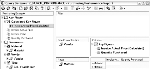
Step 1. Create a new query in BEx Query Designer to display the invoice actual price and quantity. In the BEx toolbar, click on the Open button and choose Query from the drop-down menu. In the pop-up window that follows, click on the New button. Select the InfoCube and double-click on it. In the next screen, drag and drop the Vendor and Material characteristics to the Free Characteristics and Rows sections (Figure 5).

Figure 5
Create the query
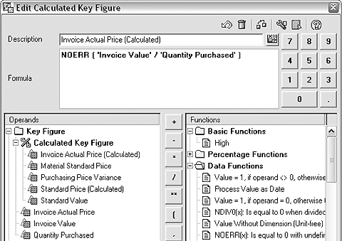
Although Invoice Actual Price could be available in the InfoCube, it is not used directly in this query. Instead, use the NOERR function (invoice value/quantity purchased), because it ensures that you do not get any errors if no quantity has been purchased. You thereby avoid division by zero overflow.
Right-click on the Calculated Key Figure subtree and select New Calculated Key Figure. Double-click on the NOERR function from the Data Functions subtree (Figure 6) to create the calculated key figure from the relevant key figures. Drag and drop Invoice Value and Quantity Purchased into the formula and insert the division sign (/) between them.

Figure 6
Invoice Actual Price (Calculated) as a Calculated Key Figure
Drag and drop the Invoice Actual Price (Calculated) and Quantity Purchased key figures to the Columns section. You should end with a screen similar to Figure 5.
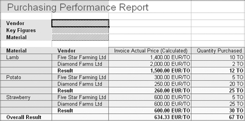
Step 2. Run the query. Click on the check mark icon in the upper left corner of the BEx Query Designer screen to run the query and view the results in Microsoft Excel. Figure 7 shows the Purchasing Performance Report drilled down by material and vendor using the query navigation functions.

Figure 7
Purchasing Performance Report drilled down by Material and Vendor
Double-click on the cell to the right of the characteristic name (for Vendor, the cell selected in Figure 7) to add drill-down by this characteristic. You could reach the equivalent result by right-clicking on the same cell and choosing Add drilldown from the context menu. My report has a default drill-down by material; therefore, all I need to do is double-click on the cell to the right of Vendor after the initial query execution.
By using division in the formula for the Invoice Actual Price (Calculated), the weighted average aggregation method works for the Result rows (and at the material level) and the unit of measure is also present.
Step 3. Add the material standard price to the report. First, I’ll show you what happens if you simply add the standard price as an attribute of material in a formula variable. In BEx Query Designer, create a new calculated key figure by right-clicking on the Calculated Key Figure subtree and choosing New Calculated Key Figure. In the next screen, shown in Figure 8, right-click on the Formula Variable subtree and choose New Variable.

Figure 8
Select New Variable from the Formula Variable subtree
You now need to make entries on several screens, as shown in Figures 9, 10, and 11.

Figure 9
Select Replacement Path to indicate you are using an attribute

Figure 10
Select Replacement Path to indicate you are using an attribute

Figure 11
Select Attribute Value and then select the exact attribute (Standard Price in this case)
Step 4. Build the calculated key figure material standard price. As in step 3, right-click on the Calculated Key Figure subtree and choose New Calculated Key Figure. Expand the Formula Variable subtree and double-click on the variable you created in step 3. Add this calculated key figure to your report.
Execute the report and drill down by vendor using the query navigation functions. The report shown in Figure 12 displays the results.

Figure 12
Drill down by Vendor
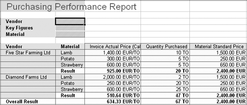
Recall that the invoice actual price is the invoice value divided by quantity purchased. The material standard price is simply the sum of the prices of the underlying materials, which is clearer if you add drill-down by material, as shown in Figure 13.

Figure 13
Drill down by Vendor and Material
Note that the material standard price is displayed as EUR, giving you no information about the unit of measure. You must build a formula that gives you appropriate overall results and enables you to list the unit of measure for the material standard price.
Step 5. Create the standard value formula that represents the value of purchased materials at material standard price. Because it is a value, you want only the currency attached to it, which is why the quantity is put in this formula as a value without dimension. The formula should look like this: Standard value = material standard price x NODIM (quantity purchased).
The trick about this key figure is the setting Time of Calculation to Before Aggregation. This setting ensures that you get the sum of products of prices by quantities. In BEx Query Designer, right- click on the Standard Value calculated key figure you just created and choose Properties. In the Aggregation section, for Time of Calculation, select Before Aggregation from the drop-down list.
Step 6. Define the material standard price. All you need to do is to divide the standard value by quantity, as shown by this formula: Material standard price = NOERR (standard value/quantity purchased).
Follow the instructions outlined in step 1 to create the material standard price calculated key figure shown in Figure 14.

Figure 14
Define the material standard price
You might be surprised by the last two calculated key figures I created. First, the material standard price is multiplied by quantity, and then it is divided by quantity again. Setting the Time of Calculation to Before Aggregation effectively puts the weighted average formulas in place.
Step 7. Build the PPV formula. As a last step to calculate the PPV, build another formula. Again, follow the steps outlined in step 3 to define the PPV: PPV = standard value – invoice value (Figure 15).

Figure 15
Define the PPV
This calculated key figure puts in place the definition of PPV. Now drag and drop the above key figures, material standard price, and PPV into your report and see what it looks like at the different levels of drill-down. Double- click on the gray cell to the right of the characteristic name to execute the different levels of drill-down shown in Figures 16 through 19.

Figure 16
Drill down by Material

Figure 17
Drill down by Vendor

Figure 18
Drill down by Material and Vendor

Figure 19`
Drill down by Vendor and Material
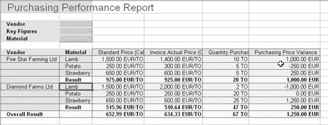
The PPV figures in the purchasing performance reports show that you save money on your purchases of strawberries and you do not gain or lose money on your purchases of lamb. However, you lose money on your purchases of potatoes. In addition, although both vendors have positive PPV, Five Star Farming Ltd. is more attractive than Diamond Farms Ltd. because Five Star Farming Ltd. has a total PPV of 1000 EUR, while Diamond Farms Ltd. has a PPV of 250 EUR.
Note that the PPV displayed in the screenshots above is consistent with the original PPV formula: PPV = (material standard price – invoice actual price) x actual quantity purchased.
This is true at all levels of drill-down and with any combination or sequence of drill-down characteristics. I achieved this result because I used the weighted average aggregation method for both material standard price and invoice actual price.
Important Points to Consider
Here are some important points to consider when choosing to use the weighted average aggregation approach.
- The Before Aggregation calculation time can produce a warning when analyzing query performance in RSRV because this setting affects the performance of the report. However, it is a standard feature and it should be used where appropriate. Avoid using it when many records are involved in the aggregation (e.g., non-cumulative key figures) and make sure it is properly tested on production volumes of data.
- If no quantities have been purchased, both actual and standard prices are displayed as zeros.
- If the material standard price attribute already exists for a material, its default aggregation could be already set to Average. Such attributes cannot be included in the formulas in this article, because mixed aggregation is not allowed in formulas and there is no way to change the aggregation method once the InfoObject has been created. In this case, you must create a copy with summation aggregation.
- If the currencies or units of measure used in aggregated prices are different, the system cannot produce a consistent result. In this case, the system displays the default asterisk symbol for Mixed Values. You can change this symbol in transaction RSCUSTV4. If you still need to display the resulting price, select the Mixed Values option in the same transaction.
Andrey Bondarev
Andrey Bondarev is a senior BI consultant for Bluefin Solutions, a UK-based SAP partner. Andrey has more than five years of experience in many areas of SAP BW, specializing in data modeling and performance optimization.
You may contact the author at andrey.bondarev@bluefinsolutions.com.
If you have comments about this article or publication, or would like to submit an article idea, please contact the editor.

