Learn the technical underpinnings and practical steps needed to use the new SAP BW 7.4 HANA Analysis Process. This new tool improves on and complements the existing Analysis Process Designer (APD) as a way to execute data-mining algorithms and stored procedures using the power of SAP HANA via an SAP BW interface.

Key Concept

The SAP HANA Analysis Process tool is an SAP BW 7.4 feature for customers running SAP BW on SAP HANA. It allows the SAP BW modeler access to powerful predictive analysis (data mining) algorithms and stored procedures that execute on the database, not in the application server as was the case with older SAP BW Analysis Process Designer tool. The previous versions of SAP BW the Analysis Process Designer (APD) was the go-to tool to perform data-mining tasks in SAP BW. Now, for companies running SAP BW on SAP HANA, the new SAP HANA Analysis Process tool that comes with SAP BW 7.4 can execute more complex algorithms faster. I discuss how to better use (and understand the reasons to use) data-mining algorithms, and give an overview of the older APD tool. I then discuss the new SAP HANA Analysis Process (HAP) tool, how to create and execute a HAP, how to tie a HAP with an APD, and scenarios where this would be required. First, here’s an overview of the way data mining used to work in SAP BW, and how it now works using the new SAP HANA Analysis Process tool.

Data Mining in SAP BW: The Old Way

For many years SAP BW has included a toolset to make using some basic data-mining models easier when running them with the data in SAP BW InfoProviders. This toolset was a combination of the data-mining workbench (transaction code RSDMWB) and the APD (transaction code RSANWB). The data-mining workbench provided the user with a method for setting up the specific parameters needed by a specific math model, while the APD allowed the user to feed InfoProvider data to the model and output the results. These results could be pushed to many places. 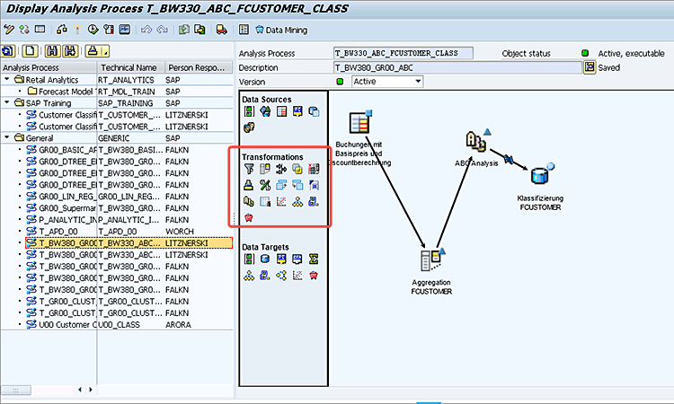One sophisticated option was to push the results to SAP CRM so they could be used to influence buying behavior and to help route inbound calls. Another common option was to push the results of the algorithm to an SAP BW InfoObject to populate an attribute. An example of this would be using the ABC data-mining model to calculate the customer’s ABC code (A= great customer, B= medium customer, and C = low-revenue customer) and put it into a navigational attribute of the customer InfoObject. Yet another example would be to target the output to a direct update of the DataStore Object (DSO), where the output of the model (in this case ABC) could be evaluated. An example of this scenario (e.g., using the APD execute the ABC data-mining model and writing the records to a direct update of the DSO) is shown in Figure 1. For companies running SAP BW on SAP HANA, setting up a data-mining model using transaction code RSDMWB and executing it with the APD is the “old way.” That is not to say that the APD itself goes away. It has a lot of other functionality designed to manipulate data that a business analyst might desire. These transformation functionalities include filtering, sorting, aggregating, and others represented by the icons in the transformations section (boxed in red in Figure 1).

The New Way to Do Data Mining: Introducing the SAP HANA Analysis Process Tool

SAP HANA (as you probably know by now) is a columnar, memory-based database. What that means is that unlike traditional databases, where the data is stored and initially accessed from magnetic disks, SAP HANA stores its data in RAM, and just uses the disk for the purposes of backing up the data. This is because RAM memory is much faster, but it can lose the data in the event of a power failure and thus needs a back-up. Other benefits of SAP HANA are that it provides fuzzy-text searching (finding what you're searching for even if it's misspelled), features to support geospatial calculations, graphical data modeling tools, a web server to serve up HTML pages, and, last but not least, support for Predictive Analysis (data mining) as part of  its application function libraries.    

Technically called the Predictive Analysis Library (PAL), SAP HANA can efficiently process data-mining algorithms that are written in R language. This programming language is the one that 99 percent of math gurus who think up complex statistical models use. By having native support for R, SAP HANA provides access to most of the data-mining algorithms written recently by academics and professionals in the field. SAP HANA also delivers many sophisticated data-mining models as part of its PAL that don’t have to be imported via R; for example, Association Analysis and Decision trees and many more. This combination of access to open source R algorithms with pre-delivered SAP HANA PAL algorithms give modelers much more flexibility than was provided by the old way.

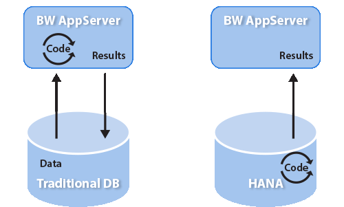
  In addition, another important feature of the new SAP HANA PAL versus the older SAP BW APD/DMWB combination is where the algorithm is executed. In a traditional client server environment, application servers (SAP NetWeaver running SAP ERP Central Component [ECC], SAP BW, or CRM) would request data they needed from a database server running on Oracle or a SQL Server. Then, once the system received the required data, it would run ABAP-based logic (in this case, the data-mining algorithm). With SAP HANA (or, in this case, SAP BW running on SAP HANA), the SAP BW application server merely triggers the process. The data is not actually moved to the application server. Rather the process is mostly done on the database server. Figure 2 illustrates how this works. Data-mining algorithms are normally very complex in nature. With SAP HANA these algorithms that literally took days to run 20 years ago now run in a matter of seconds. For companies that run SAP HANA without SAP BW, there are two ways to execute data mining. One is by using code and calling the algorithms via a stored procedure. The other is by using the Application Function Modeler (AFM). The AFM provides a graphical interface to feed data to the model and push the results to another table in SAP HANA. (This second method is the subject of a future BI Expert article.)

Using PAL with SAP HANA: SAP HAP

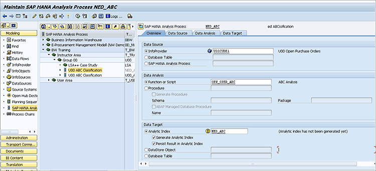
For companies running SAP BW on SAP HANA, HAP is the new tool of choice for data-mining execution. HAP provides an easy interface to perform the basic tasks of feeding data to a model, setting the model parameters, and then exporting the results. The access for building an HAP is right on the main SAP BW data warehousing workbench(transaction code RSA1). To create an SAP HANA HAP, execute transaction code RSA1 then click the SAP HANA Analysis Process link (on the left side of transaction code RSA1) .Then use the context menu in an InfoArea folder to choose Create SAP Hana Analysis Process. This opens a screen (not shown) where you can assign a name and description to your HAP. After doing so, you arrive at the Maintain SAP HANA Analysis Process screen shown in Figure 3. The first screen in the HAP is the Overview tab. It contains the guts of the HAP, including the source of the data, the specific algorithm to be executed, and where to send the output. In my example I have provided an SAP BW InfoCube (U00CUBE1) as the source data as that contains the sales information for each product. For the analysis to be performed on the data, I chose 0BW_OPER_ABC (the ABC analysis model). Finally, I targeted the output to an Analytic Index called NED_ABC. Going into more detail, the options for the Data Source could be a database table (anywhere in SAP HANA) or, more interestingly, the output from another SAP HANA Analysis Process. This latter option will be needed as more data-mining algorithms are included that might involve a two-step process where the algorithm needs a training phase and a predictive phase. Training involves running data with known results through the algorithm of the model to generate the parameters it needs to then run a second predictive phase. In this predictive phase you input data for which you do not know the results (Will customer XYZ buy from us?), and let the model’s algorithm provide a statistical prediction. 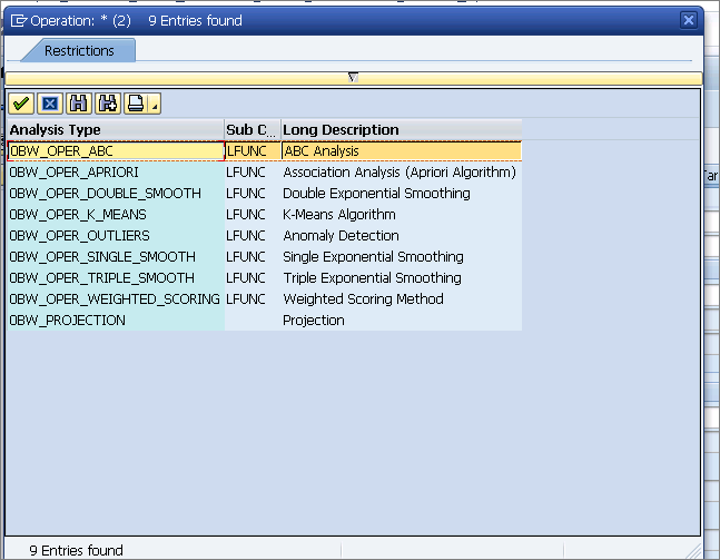In the Data Analysis section (Figure 3), you can execute various PAL functions. A list of some that are on my system are shown in Figure 4. (These functions can be selected via the drop-down field next to the Function or Script radio button in Figure 3.) In my example, I chose the first option in the list—BW_OPER_ABC—which is the ABC analysis option. Although it is possible to access more data-mining choices, they need to be installed on the underlying SAP HANA database. To find out more about these PAL functions and the available algorithms, click this link: The last setting on the Overview tab screen is the Data Target area. In my first example I have set this to an Analytical Index, which is basically an SAP HANA table that is exposed to SAP BW as a transient InfoProvider that can be queried using BEx Query Designer. The DataStore Object and a Database Table options in SAP HANA are fairly straightforward. Another option is the Embedded in Data Transfer Process radio button, which I have selected (Figure 5). I discuss this last option later on in this article. 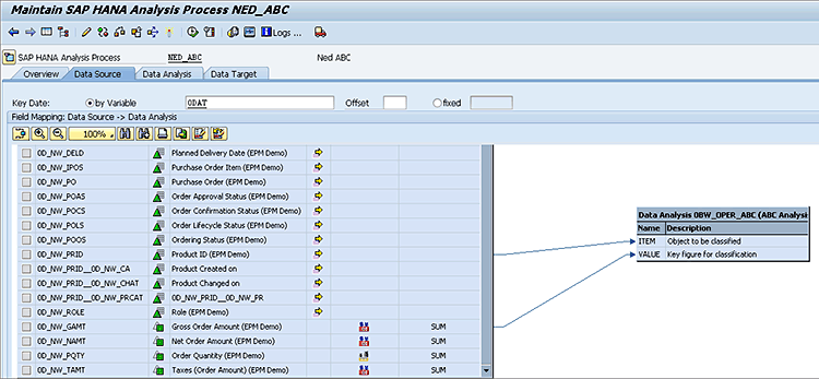Next, click the Data Source tab in the HAP tool (Figure 6). Here you map the fields from the source (the U00CUBE1) to the fields required by the model. In the case of ABC analysis it is very easy as the model needs just two parameters: What you want to ABC (for example, customers, products, or cost centers) and what measure (key figure) you want to use to rank by. In my example, I have mapped the product ID to the ABC model’s ITEM and the Net Order Amount (which should all be in the same currency) to the model’s VALUE field by dragging and dropping (as you normally do with SAP BW transformations). The Key date field would apply only in the event of time-dependent master data, which is not involved in this scenario, so the default, ODAT, is not used in this situation, but leaving it on the screen does not cause any issues. 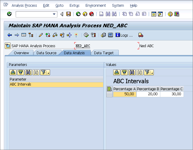Next, click the Data Analysis tab (Figure 7). This tab contains any settings or parameters that the data mining algorithm might need. In the case of the ABC analysis example I have the model find the products whose values equal 50 percent of the total value of all the products and then make these products A products. Similarly the next best-selling group, the Bs, are the additional products that provide 70 percent of the total value (50 + 20). All the remaining products are Cs. 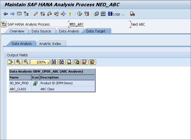The last tab is the Data Target tab (Figure 8). The options in this tab change depending on the options you picked for the target way back in Figure 3. In this example, since the system is creating an analytical index, the Analytic Index subtab just shows the fields that are in this automatically generated table. If your target was a DSO or an SAP HANA table, you would need to map the output of the model to the fields on the DSO or SAP HANA table. Since the target is an Analytic Index, another subtab and set of sub-subtabs are created (shown in Figures 9, 10, and 11). The first one just shows the technical name (@3NED_ABC) of the generated transient InfoProvider as well as the InfoArea folder where you would look for the InfoProvider when you want to write a query against it in the BEx Query Designer. 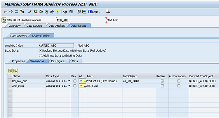Figure 9 shows the second Analytic Index subtab—Dimensions—in more detail. Here you can map BW InfoObjects to the dimensional fields in the analytic index. In this example, I entered 0D_NW_PRID in the InfoObject column to map to a field with the same name. Doing this gives the query designer access to the master data of this InfoObject that is already stored in SAP BW. The next subtab is Key Figures. I do not show a screenprint of this subtab, but in the same manner that you use the settings in the Dimension subtab (Figure 10), in the Key Figures subtab, you create mappings to BW objects. Specifically, you can map the measures in the analytic index to the SAP BW InfoObjects of the key figure type. This is normally not needed but you might do it if some SAP BW security is tied to the InfoObjects key figure. In that case, they would need to be mapped. 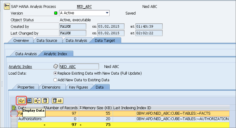The final subtab is the Data tab for the Analytic Index (Figure 11). After normal SAP BW activation and execution (using the matchstick and execute icons, respectively, at the top of Figure 10)you can see the results in the Analytic Index without the need to run a query against the auto-generated transient InfoProvider. If you click the display data (eyeglass) icon (shown in Figure 11) you can examine the results of the ABC model’s algorithm. This result is shown in Figure 12. Once in this screen click the execute icon to generate the output, which is shown in the bottom portion of the figure. In these results, although not all the records are shown, you can see that only a small number of the high-revenue customers have been coded with an A, with the majority of customers receiving a C rating.

Advanced Options with HAP

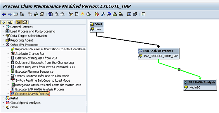
Although I have summarized the basics of HAP, there are a few more points I want to mention for the more advanced SAP BW user. The first one is that you can schedule the execution of HAP via a process chain. Additionally, if you output the HAP to a persistent DSO or SAP HANA table, these results could then feed into the older APD for further manipulation that can’t be done by HAP, for example filtering. Both the HAP (the first step) and the APD that further processes the HAP (the second step) can then be scheduled in a multi-step process chain as shown in Figure 13. The final point I would like to address is the HAP Embedded in Data Transfer Process option I mentioned earlier. In this scenario (Figure 14) I select the Embedded in Data Transfer Process radio button. If this option is set, then you merely need to activate the HAP but not execute it. Rather you need to build a transformation and a Data Transfer Process (DTP) to take the results from your model and populate another SAP BW target via a DTP. The first step in using the HAP’s output is to create a transformation. Figure 15 shows the new source option for creating a transformation. You guessed it, an SAP HANA Analysis Process. In this case I have the target of the transformation updating SAP BW InfoObject 0D_NW_PRID, as I want to populate the ABC code as a navigational attribute of the product master. 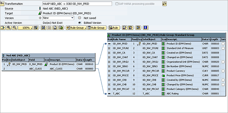In this specific case the needed transformation is simply the model outputting the part number (PRID) and the ABC code, so I just need to map these to the corresponding fields on the InfoObject, as shown in Figure 16. 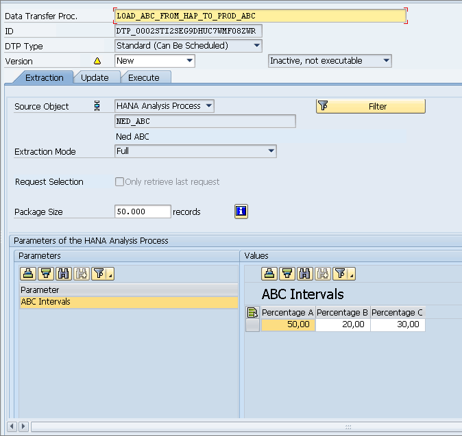Now, the last steps are just to create and then execute the DTP. This DTP first runs the HAP and then pushes the data through the transformation and into the InfoObject, as shown in Figure 17. It is important to note the DTP (Figure 17) allows you to set the specific ABC parameters you desire. Thus different targets could contain different values for ABC if you change the percentages. 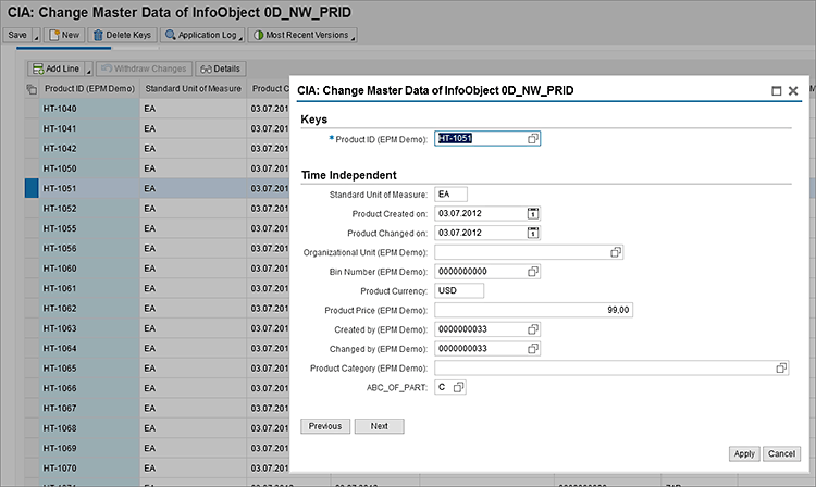After executing the DTP the final step is to prove that it works. You can use your basic knowledge of SAP BW to display the master data as I did Figure 18 for the product and review the data for a specific product. As you can see (boxed in red) the ABC code is populated for the product. To learn more about HAP and to try it out, consider taking the SAP BW on SAP HANA training class: BW362.