This is the first article on a series on buffer & safety stock planning within SAP S/4 HANA (also for SAP ECC). It shows a variety of features to optimizer safety stock planning, explaining all the methods and showing some small add-on solutions.

Static Safety Stock

The safety stock specifies the quantity that is to cover an unexpectedly high requirement in the coverage period. Its task is to reduce the risk of shortfall. In the material master, the MRP controller uses his or her experience to define a fixed safety stock that is to reduce the quantity available for MRP. This is a static safety stock because its level can only be adjusted manually to changing demand quantities and the safety stock level can only be adjusted manually in time. The static safety stock is therefore active for all future periods. The static safety stock is therefore time-constant and is generally not available for planning – this is a basic characteristic of the safety stock that it is not available for planning purposes. This means that as soon as the safety stock is fallen below the safety stock level, MRP will replenish the missing safety stock. There are exceptions, which I will explain later. Defining a safety stock means that a planned order or a purchase requisition is always triggered in MRP as soon as the stock falls below the safety stock level. The term “not available for planning” means that the safety stock is not used to cover requirements from the point of view of MRP. However, it is not contrary to the fact that it can still be used to meet unexpectedly high demands. In manual reorder point planning, you can enter a safety stock value in the material master record. However, this is for information purposes only. In automatic reorder point planning and forecast-based planning, the system automatically determines and adjusts the safety stock value as part of the forecast. But even the safety stock is only an optional parameter in reorder point planning, it is very important to maintain it because it gives you later in the MRP process an Alert if the inventory falls below safety stock. That is like the fuel display in your car. If you run on reserve, the car gives you a red light on your fuel display. And that is exactly the reason, which you should always maintain a safety stock. If the inventory falls below the reorder point or the safety stock the system flags the corresponding material for MRP by creating a planning file entry. If the material master record is newly created, the safety stock must always be entered manually in the Safety Stock field in the Net Requirement Calculation area on the MRP 2 tab page of the material master, even if it is later overwritten by the SAP system (see Image 1). This makes it possible to plan a material even if no forecast calculation has yet been carried out. To do so, in the SAP Menu, choose Logistics > Materials Management > Material Master > Change Material > Immediately and switch to the MRP 2 view. 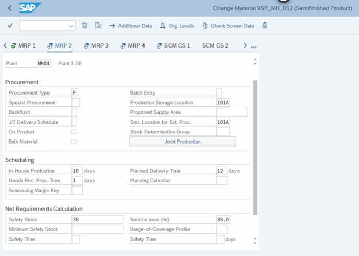[caption id="attachment_77519" align="alignnone" width="703"] Material Master: MRP 2 Tab[/caption]

Static Safety Stock available or not available for MRP

For each requirement that leads to a shortfall in the stock available for MRP, requirements planning creates a procurement element to procure the difference. The safety stock reduces the quantity available for planning (see Image 2). Requirements planning fills the safety stock again when it falls below this level, as indicated by the receipts in Image 2. This is also the case if the safety stock is only fallen short of by a small quantity in relation to its level. This type of safety stock is independent of the requirement quantities and is therefore static. The safety stock is displayed in a separate row in the current stock/requirements list and in the MRP list. 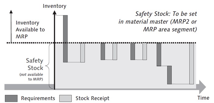[caption id="attachment_77520" align="alignnone" width="703"] Example of Safety Stock Available for Planning and Safety Stock Not Available for Planning and the Corresponding Receipts (Source: SAP)[/caption] If the safety stock is only fallen short, e.g. of 1 or 2 pieces in relation to its inventory level of e.g. 1000 pieces, or the minimum lot size has a big amount, it should create immediately a big planned order or purchase requisition. Therefor the portion of the safety stock available for planning can be defined for each MRP group in Customizing (see Image 3). It is defined as a percentage based on the safety stock level specified in the material master. To do so, in SAP Customizing, choose Implementation Guide > Production > Material Requirements Planning > Planning > MRP Calculation > Stocks Define Availability of Safety Stock. 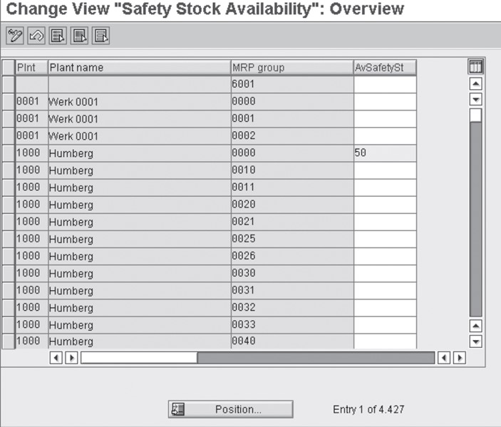[caption id="attachment_77521" align="alignnone" width="703"] Customizing: Availability of Safety Stock[/caption] A new order proposal is not generated until the available portion of the safety stock is fallen short. This is used to fill up (at least) the safety stock, as shown by Image 4. As a result, no separate order proposals are generated for very small shortages. This reduces the administrative effort and calms planning. This is an enormous advantage in inventory management to make more effective use of safety stocks and achieve inventory reductions. 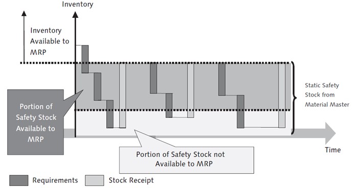[caption id="attachment_77522" align="alignnone" width="703"] Partially Available Safety Stock (Source: SAP)[/caption]

Automatic calculation of static Safety Stock

This method is used in particular in automatic reorder point planning and forecast-based planning (consumption-based planning procedure), but can also be used in MRP. When you use the automatic safety stock, the reorder point and the safety stock are calculated automatically at the frequency of executing the sales forecast, resulting in a moving reorder point and safety stock over a longer planning period. The more the following assumptions apply, the better the results of the automatic safety stock method:

• There is a regular demand.
• The relative forecast error is the same in the past and future.
• The mean value of the forecast error is as low as possible.
• The forecast error is distributed approximately normally. This is because the safety factor is calculated on the basis of a normal distribution of the forecast error.

The automatic safety stock depends on 3 main influencing factors:

1. the service level specified in the material master record (MRP 2 view)
2. on the accuracy of the forecast
3. and the Replenishment Lead Time (MRP 2 view)

In the following these factors will be described.

The influence of Forecast Accuracy and the Service Level under the Normal Distribution to buffer levels

Demand is an important factor influencing safety stock. Customer demand is generally subject to random fluctuations that can be reflected by probability distributions. In the case of normally distributed demand quantities, the most probable value of demand quantities is exactly the middle of the scale of all possible demand requirements. Since this value is used in the formulas for determining requirements, only 50% of all requirements can be covered, that is, only a service level of 50% is saved. Therefore, the main task of safety stock is to cover the demand requirements beyond the most probable value or to limit the risk of a lack of service. Due to the relationship between safety stock and missing quantity costs described above, when deciding on the safety stock level, you must analyze the cost-related and revenue-related consequences of non-delivery or delivery disruptions and compare them against the costs for retaining safety stocks. The service level can therefore be interpreted as a one-sided statistical security if normal distribution to Gauss (see Image 5) is assumed. 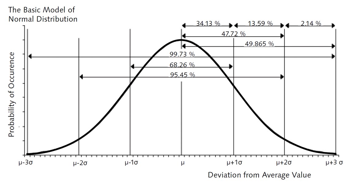[caption id="attachment_77523" align="alignnone" width="878"] Normal Distribution by Gauss[/caption] The basic idea of normal distribution is that the further away this state is from the mean value (m), the more likely the occurrence of a particular condition (characteristic value) is more unlikely. The measure here is the variance (s). The Gaussian Bell Curve (Gaussian Normal Distribution) illustrates this behavior. The curve shown in Image 1 describes the occurrence of all possible states, that is, a probability of 100% (that is, any stock on hand is always found). A status can therefore be the occurrence of availability or non-availability. The nature law discovered by mathematician Gauss now states that the probability of a characteristic value occurring between the mean value (m) and the mean value plus a variance (m + s) is just 34.13%. The probability that a characteristic value is between m and m + 2s is 47.72%, and the probability that a characteristic value is between m and m + 3s is 49.865%. Half of the symmetric curve is always exactly 50%. The fact that a characteristic value is between m – s and m + s has a probability of 68.26%, and the probability of a result between m – 2s and m + 2s is 95.45%. This lawfulness applies regardless of the individual case in question. Normal distribution is a basic element of a warehouse management strategy. The normal distribution is not always applied in practice. On the other hand, the case of variances in normal distribution is increasingly used there. If smaller quantities are ordered more often, the warehouse stock tends to return around a mean value, which results in a smaller variance (see Image 6). If you order less frequently, but a larger quantity for each purchase order, this results in greater deviations from the mean value and therefore a larger s value. 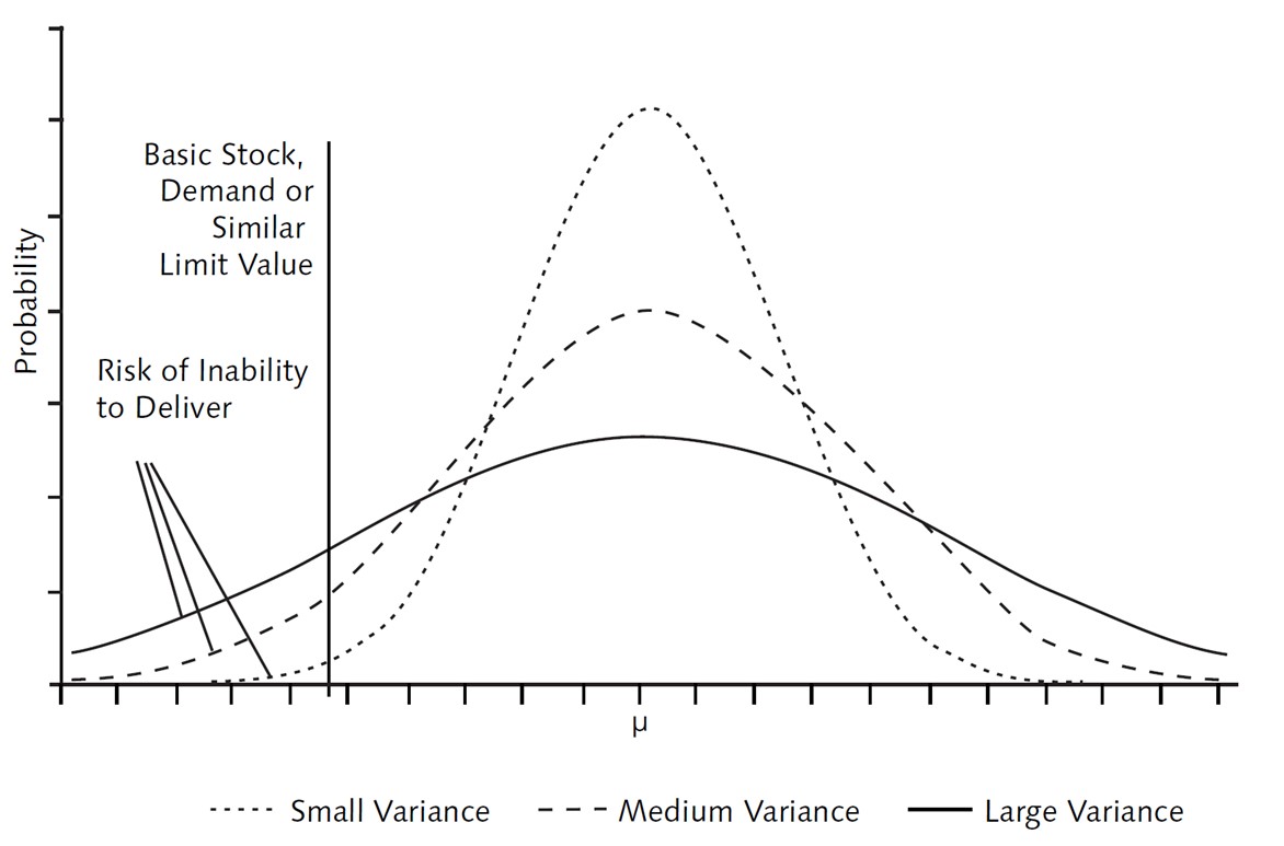[caption id="attachment_77524" align="alignnone" width="914"] Normal distribution with variances: small variance (large amplitude), mean variance (mean amplitude), and large variance (small amplitude)[/caption] Assuming that the forecast of future requirements is distributed normally, with a mean forecast error of 0, you can determine a safety factor r (z value) that guarantees the desired service level. In Table 1, you can see the safety factors that result from the normal distribution for the respective service level.

Service Level	Safety factor r
50.01%	0.0003
80.00%	0,8416
90.00%	1.2816
95.00%	1,6449
98.00%	2.0537
99.00%	2,3263
99.50%	2.5758
99.90%	3.0903
99.99%	3.7191

Table 1: Security factors by service level (source: SAP)

Measurement of forecast quality with the SAP add-on Forecast & Monitoring Tool (FMO)

To continuously measure the quality of the forecast, SAP has developed another add-on for SAP S/4HANA and SAP ERP that introduces the Forecast & Monitoring Tool (transaction /SAPLOM/FMO).

The Replenishment Lead Time as an Influencing Factor

The replenishment lead time is influencing the safety stock as well as the reorder point. The reorder point is defined as the sum of safety stock and forecasted demand within the replenishment lead time (see Image 7). [caption id="attachment_77525" align="alignnone" width="922"] Reorder Point and Safety Stock in Relation to Replenishment Lead Time[/caption] When the material is withdrawn, the static availability is checked against the reorder point, that is, the availability at the current time without taking the future into account. To do this, the remaining stock is compared with the reorder point. If the stock is smaller than the reorder point, the material is flagged for MRP. During the next planning run, a purchase requisition or a planned order is generated automatically for the corresponding material. If the reorder point is too small, that is, less than the following requirement, an out-of-stock situation must be expected, as shown in Image 8 on the left side. In individual cases, this means that a sales order cannot be delivered. In this case the average forecasted demand was not calculated correctly or the replenishment lead time was too short. If the reorder point is too high, there are usually overstocks, but this is often not even notice at all (on the right side of Image 8). In this case the average forecasted demand was not calculated too high or the replenishment lead time was shorten than expected. 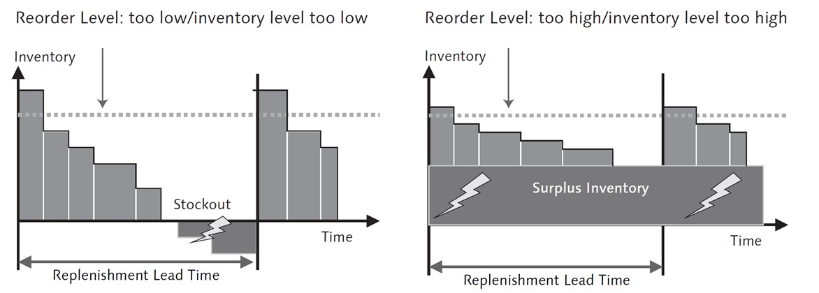[caption id="attachment_77526" align="alignnone" width="935"] Influence of Reorder Point, Left with Out-of-Stocks, and Right with Overstocks[/caption]

The SAP Formula

The SAP Formula to calculate safety stock has 3 values: Formula for Calculating Safety Stock The safety stock is calculated using the following formula: SS = r × Ö W × MAD The individual parts of the formula have the following meaning:

• W = Replenishment Lead Time (RLT)or Delivery time in days / forecast periods in periods
• SS = Safety stock
• R = Safety factor
• MAD: Mean Absolute Deviation of Forecast

The Replenishment Lead Time can be calculated in different ways: Formula for RLT for In-House Production If the material is produced in-house, the delivery time is calculated as follows: Delivery time (for in-house production of material) = start period + in-house production time + goods receipt processing time In the case of external procurement of a material, the delivery time is calculated as follows: Delivery time (in the case of external procurement of the material) = goods receipt processing time + planned delivery time The delivery time is specified in workdays. The forecast period is read from the material master record and is specified in periods. That means the mean absolute deviation (MAD) has to be converted to days. MAD is a forecast accuracy statistic. This is explained later. The factor R describes the safety factor for a specific service level (SL). The safety factor is calculated from the service level of the product master. It specifies the number of standard deviations that are necessary for a certain service level. Is For B. If a service level of 99.5% is notified, the value of the safety factor (R) must be "3.2". This is an alpha delivery readiness level. The mean absolute deviation represents the absolute deviation between the forecasted and actual requirement quantities. It is a key figure for the forecast accuracy of univariate forecasting techniques. The system uses two different formulas to calculate the MAD. The MAD for forecast initialization is calculated using the following formula: The individual parts of the formula have the following meaning:

• Vt = Actual consumption in period t
• Pt = forecasted consumption in period t
• n = Number of underlying values

After the MAD has been initialized, it is smoothed in each of the following ex-post forecast periods using the smoothing factor () as follows:

Formula for MAD

MAD(t) = (1–) × MAD( t – 1) + × |V(t) – P(t)| The default smoothing factor in the SAP system is 0.3. When this factor is used, the MAD of the previous period, MAD (t – 1), is weighted at 70%. The current absolute deviation between the consumption value and the forecast value is 30% included in the new MAD. The execution of the ex-post forecast is a means of checking forecast accuracy, which is always carried out by the SAP system when sufficient historical data is available. This case always occurs if the number of historical values specified in the material master that the system is to take into account during the forecast exceeds the number of initialization periods to be taken into account. The ex-post forecast makes it possible to make a statement about how well the forecast method used anticipates the development of demand in the past. This provides initial indications of how well the corresponding forecasting technique is suited to predicting future demand. One disadvantage of the ex-post forecast is that it can only be carried out for certain forecast methods. The question arises as to the period over which the MAD is to be calculated. This period can be set using a parameter to B. structure breaks in the demand time series. If no value is specified here, the system uses all saved historical values. Values up to the number 60 can be saved here, for example: B. 60 days, 60 weeks, or 60 months. These forecast values are calculated according to the frequency of forecast execution, which is defined by the period indicator in the material master. Accordingly, the safety stock is also recalculated according to the frequency of the forecast execution, that is, the is valid for a day, week, or month. Another aspect that is expressed in formula w = is that not only the replenishment lead time but the root from the relationship between replenishment lead time and forecast period is included in the formula. This concerns the following factor, which requires further clarification:

Formula for the replenishment lead time factor

w = Ö Replenishment lead time / forecast period Depending on the procurement type, the replenishment lead time is made up of several different components. For the sake of simplicity, only the planned delivery time that generally represents the largest proportion of the replenishment lead time should be considered here. The planned delivery time is stored in calendar days in the system. However, to produce a forecast, a conversion to working days is required. Therefore, the planned delivery time of the material master is multiplied internally by 5 / 7 and then rounded to an integer value. The denominator of the above formula contains the forecast period that takes the value 5 when the period indicator W (week) is used. If you use the period indicator M (month), the system uses the value 21.4. If the replenishment lead time and the forecast period are the same (that is, w = 1), the safety stock is calculated in the same way as the standard formula for the safety stock, whereby here the MAD is included in the calculation:

Formula for Safety Stock in SAP

SB = R × MAD The safety stock resulting from the formula now covers the uncertainty of the consumption variance during a forecast period (for example, for example, a week). However, if the replenishment lead time differs from the forecast period, the safety stock level is adjusted accordingly. This is provided by the factor w, which has already been discussed. If the replenishment lead time is longer than the defined forecast period, this results in a higher safety stock and vice versa. The safety stock can be specified in the material master in the view MRP 2 in the Net Requirements Calculation field group in the Safety Stock field. To do this, in the SAP Menu, choose Logistics > Materials Management> Material Master> Change Material> Immediately and switch to the MRP 2 view. You can specify a lower limit (minimum safety stock) for the safety stock. If the calculation of the safety stock results in a lower value than this limit, the safety stock is automatically set to this minimum value. You enter the lower limit value for the safety stock in the material master record in the view MRP 2 in the area Net Requirements Calculation in the field Min. Security On. Finally, note that the reorder point can also be calculated automatically. The reorder point is defined as the sum of safety stock plus forecasted demand within the replenishment lead time (see formula w =). The calculation of the reorder point is explained using the following example. Note that the safety stock calculation can lead to rounding effects. An example of Calculation of the Reorder Point A forecast was carried out on a monthly basis. A month is based on 30 days. The forecast values are as follows:

• Month 1: 200 pieces
• Month 2: 300 pieces
• Month 3: 400 pieces
• Safety stock: 100 pieces

The replenishment lead time is 40 days, that is, a total monthly demand + a portion of the following month. The reorder point is therefore 100 + 30 / 30 × 200 + 10 / 30 × 300 = 400 pieces. (For more information or questions, contact the author at marc.hoppe@sap.com.).