In this exclusive report, take a walk into the world of SAP Predictive Analysis and how it ties into SAP HANA and SAP Lumira (formerly known as SAP Visual Intelligence). Learn the importance of general predictive modeling concepts, and then apply those concepts as part of a bigger discussion about the architecture and features of SAP Predictive Analysis. Finally, get an early peek at what’s coming for SAP Predictive Analysis in the near future.
Key Concept
A predictive model is an equation, algorithm, or set of rules used to predict an outcome based on input data. Predictive models can simply be a set of business rules based on past observations, but to develop more accurate and statistically rigorous predictions, statistical algorithms for developing the predictive equation are often used.
SAP Predictive Analysis is the latest addition to the SAP BusinessObjects BI suite and introduces new functionality to the existing BusinessObjects toolset. Predictive Analysis extends the visual intelligence offerings of SAP Lumira (formerly known as SAP Visual Intelligence) to include new predictive functionality powered by both open source R and SAP-written algorithms. Predictive Analysis was first released for general availability in mid-November 2012 (version 1.0.7), and there have been several releases in 2013 with additional functionality.
Predictive Analysis replaces SAP’s Predictive Workbench tool, which was last updated in December 2011. Predictive Workbench was a client-server tool based on the SPSS PASW modeler engine (supported by SPSS from late 2009 through late 2010). However, after SPSS was acquired by IBM in 2009, SAP was no longer able to license upgraded versions of the predictive engine, effectively mothballing Predictive Workbench.
In this detailed special report, I first provide an overview of the generic predictive modeling process before going into details about SAP Predictive Analysis modeling engines and the software’s features and functionality. I also look at how Predictive Analysis integrates with Lumira and SAP HANA.
Note
The next section of this report delves into the core elements behind predictive analytics and modeling. If you are familiar with these concepts, you can jump ahead to the section titled “SAP Predictive Analysis Prerequisites and Skills.”
Predictive Modeling Overview
Predictive models are important because they allow businesses to forecast the outcomes of alternative strategies prior to implementation and determine how to most effectively allocate scarce resources, such as marketing dollars or labor hours. Common applications for predictive models include:
- Response and uplift models predict which customers are most likely to respond (or incrementally respond) to a marketing prompt (e.g., email, direct mail, promotion)
- Cross-sell and up-sell models predict which product suggestions are most likely to result in an additional or increased sale to a given customer
- Retention and attrition models predict which customers are most likely to leave or stop purchasing in the near future and examine what interventions might reduce the likelihood of customers leaving
- Segmentation predicts which customers behave or transact similarly and might respond similarly to marketing or service offers
- Fraud models predict which transactions, claims, and interactions are most likely to be fraudulent or require further review
The common business problems addressed by predictive models are not to be confused with predictive algorithms. Each of the above problems can be solved using a number of different algorithms. Understanding the characteristics of a business problem and marrying data with the most appropriate predictive algorithm is the portion of statistical modeling that is often more art than science. For example, if a firm wants to predict a simple binary outcome (e.g., will a customer accept an offer), the modeler can employ a decision tree, naive Bayes classifier, or logistic regression model. Each of these prediction methodologies has advantages and disadvantages in terms of ease of implementation, precision, accuracy, and development complexity.
While the value of predictive modeling varies from firm to firm, it is easy to quantify the value of better predicting outcomes. From a marketing perspective, allocating scarce marketing resources to the customers most likely to respond can increase response rates and cut expenses at the same time, often with return on investment on the order of millions of dollars per year. Predictive models also allow firms to test multiple proposals in a simulation-type environment to predict outcome revenue rather than relying on gut-feel management when deciding among alternatives. For financial services or insurance firms, better predicting which customers are likely to have a claim or default on a loan allows more accurate pricing of risk and a higher likelihood of attracting the most desirable customers. Similarly, having repeatable, quantifiable business rules for creating these models allows businesses to react to market changes more quickly and rebuild models to reflect changing business environments once a shift is identified.
Typically, firms start developing predictive models for one particular area or department, and quickly identify many opportunities to apply similar applications to other functional areas.
The Flow of Data in the Modeling Process
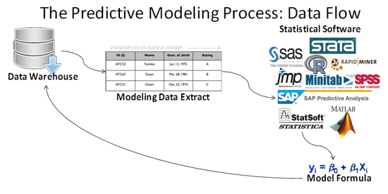
Figure 1 shows an overview of the flow of data in the modeling process.

Figure 1
The data flow behind predictive modeling
Modeled data from a data warehouse is extracted and often transformed for transfer to the predictive tool. This data transfer occurs through text file exports or direct database connections. In the best situations, the predictive modeling tool is able to access and write data directly back to the data warehouse. Often, the data transfer process is iterative, as the modeling data extract is adjusted and variables are added, deleted, or modified.
Although much emphasis is placed on the software used for prediction, running the predictive algorithms is actually only a small portion of the model building process. In fact, in marketing materials for Predictive Analysis, SAP states that generating the predictive models accounts for only 20 percent of the time and effort in the modeling process. Data manipulation, exploration, and implementation take up more resource time than actually creating the model.
Therefore, selecting a modeling tool that incorporates data exploration and manipulation elements, facilitates implementation, and integrates seamlessly with the original data source means fewer data transfers and faster implementation of the predictive insights.
At a high level, the predictive modeling process consists of the following steps:
- Step 1. Identify goals for the predictive model
- Step 2. Select an appropriate modeling tool
- Step 3. Perform exploratory data analysis and investigate the available data
- Step 4. Develop the model (including selecting a predictive algorithm and predictor variables to include in the model and evaluating model fit and accuracy)
- Step 5. Implement the selected model
- Step 6. Maintain and update the model as needed
Let’s look at these steps in more detail.
Step 1. Identify Goals for the Predictive Model
All business leaders have to face the issues that keep them up at night when considering the future of their company or industry. Identifying ways to turn predictive analytics insights into actionable business decisions is often a challenge, as analysts can become overwhelmed with summarizing and examining the data available and unable to drive actions that can produce a return on investment to the organization. An analyst, with management support, must identify goals for the analysis and a desired outcome or deliverable. This might include:
- Which customers are most likely to respond to a marketing trigger?
- Which customers might cancel their subscriptions or stop transacting soon?
- Which offers, environments, displays, or other inputs might trigger a higher purchase amount?
- Which customers might have life events that would trigger a purchase?
Answering these questions produces actionable results with a quantifiable return on investment.
Finally, in developing the goals of the analysis, the analytical and management teams must ensure sufficient data is available to build the models. For example, a company that does not have a customer database can’t develop customer segments or determine which customers are most profitable. An insurance company that wants to build a model to detect fraudulent claims must be able to provide or identify a set of past fraudulent claims. A predictive model is not a magic wand that can pull insights out of thin air; it is simply a system of rules or equations that can synthesize past experience to determine the most likely future outcomes.
Unfortunately, this part of the process is often ignored and time and effort are squandered when the modelers later determine there is insufficient data to complete the analysis.
While no tool can select the best business strategy and communicate to the analytical teams the modeling requirements to implement the strategy, easy-to-use data visualization and BI tools can help identify trends and preliminary insights to direct predictive analysis. A healthy BI practice and user-friendly query tools can identify areas for improvement and quickly assess the sufficiency of data for modeling, expediting this first step in the modeling process.
The Data Source
In addition to considering the business goals, this first step must also include a plan for obtaining the data required for the analysis. The datasets used to generate predictive insights are critical to the analytic project’s success. The modeling dataset must not only be constructed carefully, but also be a collaborative effort between the subject matter experts who understand the data, the technical team members who actually pull and build the datasets, and the analytics team members who consume the data and build models.
In the best situations, the organization has a data warehouse with data from all areas of the company loaded into a central location and in a standard format. Typically, the enterprise BI reporting system (e.g., BusinessObjects) lets business users facilitate reporting and data access. Sometimes, to ensure that data is at the level of detail required for modeling, the modeling extract must be pulled directly from the data warehouse rather than from pre-aggregated reporting marts.
Step 2. Select an Appropriate Modeling Tool
When evaluating predictive tools, modelers should consider several functional areas to ensure a tool meets their needs. The match between the modeling tool’s capabilities and the organizational requirements and budget determines which solution to select. This section summarizes key functional areas to consider during the selection process.
Data Access
As discussed previously, file creation is often the most time-consuming portion of modeling, so ensuring that the modeling tool can access the data is critical to expediting this process. Ask yourself these questions:
- How is modeling data imported into the tool?
- Can databases be accessed directly or must data be transferred exclusively though flat files?
- Can the tool write results or models back to the database?
Data Manipulation
Data manipulation includes binning, grouping, value changes, and calculations on existing data fields. If the model development process involves evaluating and potentially modifying fields in the database, this functionality may expedite the modeling process rather than having to go back and create a new extract from the source system each time. However, if these modification rules cannot be exported or documented, they have to be re-created in any system that needs to score the model.
System Architecture and Processing Capacity
Some predictive algorithms require significant processing power, often iterating through the data many times to calculate optimal models. As more data becomes available and companies want to analyze big data, ensuring that the predictive tool can process large datasets is critical. Therefore, organizations need to decide between predictive tools that are installed on a user’s local machine and those that can process data on a server. Local client tools are easy to deploy and require no dedicated hardware, but are limited in the amount of data they can process. Server-based tools typically require dedicated hardware and are more complex to install and maintain, but can process big data and allow many users to share the same resources.
User Interfaces (UIs)
Predictive tools have vastly different interfaces, varying from user-friendly, drag-and-drop functionality to code-only interfaces. Some tools do not even have an interface and can only run via batch jobs submitted remotely. Tools that are fully code based often offer more functionality and more extensive predictive libraries, but can increase development time and require more technical resources to operate. UI-based solutions can sometimes be operated by less technical resources and expedite the model development process.
Predictive Algorithms
The library of predictive algorithms available in each tool varies. While numerous algorithms exist, most organizations can perform a wide range of analysis with a limited toolset that has a few algorithms for each classification, clustering, regression, and time series analysis. However, it is important to define the goals or types of models the organization expects to build prior to selecting a tool to ensure that the selected tool has appropriate functionality. For example, if an organization is purchasing a predictive tool exclusively to develop sales forecasts, it should buy a tool that specializes in that area with special features to accommodate seasonality and periodic events, whereas a company planning to perform customer analysis would want a variety of tools, such as clustering, decision trees, and possibly regression algorithms.
Model Evaluation Features
Evaluating models and comparing alternatives is key to selecting the final model. Tools that assist analysts in comparing alternatives speed the development and selection processes. Model evaluation tools include automated visualizations for things such as lift charts, residual analysis, and confidence intervals on the coefficients and predicted values.
Model Implementation and Maintenance Features
Once a model is selected, most organizations want to deploy it as quickly as possible. Depending on the organizational needs, this may simply be attaching the model score to a small set of data. However, in many instances the organization requires the ability to call the scoring model on demand, which requires writing the scoring algorithm (rather than just the score values) back to the database. Predictive tools that can publish algorithms back to the database as a stored procedure or function call or be encapsulated in a callable block of code expedite this process. Depending on the complexity of the scoring algorithm, calculating the coefficients and programming the scoring function can be time consuming. Additionally, if the data has been manipulated within the modeling tool, being able to export those rules or include them in the scoring algorithm significantly expedites the implementation process.
The Predictive Marketplace
While the popularity of predictive tools is exploding, software providers are struggling to keep up with increased user demands for data processing power and increased functionality while maintaining usability. Wikipedia maintains a relatively complete
comparison of statistical packages. Additionally, blogger Robert A. Muenchen has written an article on the
popularity of data analysis software that monitors the use of different tools in the marketplace; his research indicates that the R programming language is one of the top statistical packages used by those performing predictive analytics, and R’s use has been growing rapidly over the past several years. Commercially available software is more frequently used by business organizations. However with the licensing costs of some popular software packages increasing and the influx of recent graduates with experience in open-source languages, many organizations are moving to open-source tools, such as R. I have more to say about R later in this report.
The following is a list of characteristics an organization should consider when selecting a tool for a new analytics venture. Once it identifies the analytic goals, the organization should determine which tool provides the best match to the project’s needs and the long-term goals of the organization.
Algorithm-Specific Tools
While many tools try to have a full suite of algorithms available, there are several tools available with a narrow focus that attempt to perform one algorithm or one subset of algorithms very well. These tools often offer usability and visualization features that surpass full-function tools, but are only used for one type of algorithm, such as decision trees.
Full-Function Code-Based Tools
The most comprehensive tools, which offer access to the largest range of diagnostic tools and modeling algorithms, generally require users to have in-depth knowledge of both statistics and coding. These tools are often also fully-functional coding languages and, therefore, can be used for all the required data processing and manipulation, and for programming any algorithms that are not already included in the code library. These tools offer significant flexibility in terms of data preparation, predictive algorithms, and model evaluation, but suffer from lack of usability, a high learning curve, and difficulty to generate visualizations.
Cloud Solutions
The most recent market entrants are offering predictive-in-the-cloud solutions with Web-based modeling interfaces, cloud-based data storage and processing, and a pay-per-byte or pay-per-score model for data storage, model building, and prediction.
Step 3. Perform Exploratory Data Analysis and Investigate the Available Data
The data exploration process involves evaluating all the data elements available for modeling and determining which elements to include in the analysis. This includes examining the distribution of values within an attribute, learning how they relate to the response variable, and evaluating the quality of each attribute. For example, do values look reasonably accurate? For what percentage of the observations is this variable populated? Is the data spread across possible values?
This work may involve building new variables or changing the definitions of existing variables. This exploration process should result in a short list of high-quality predictor variables.
Step 4. Develop the Model
A modeling dataset is often structured differently from how data is typically stored in a data warehouse or reporting mart. Therefore, much of the time and effort in the modeling process is spent designing, calculating, and testing the data extract. In marketing materials for Predictive Analysis, SAP indicates that data access and preparation steps account for 36 percent of the total time spent on model development.
In reality, pulling the modeling dataset is an iterative process, and the timeline of the modeling process can be extended significantly if a new file must be imported each time a change needs to be made to a predictor field. Tools that have direct connections to the source data or allow manipulation of the input file within the modeling tool can significantly cut down on the data preparation portion of the modeling process.
The format of the modeling dataset depends on the desired outcome and the input requirements for the modeling algorithm used. For example, if the goal is to forecast daily sales for Store A, the data must be aggregated to the daily level for only Store A prior to being fed into the predictive algorithm. Similarly, to predict a customer’s likelihood to purchase, the data must be at the customer level — for example, one row per customer, with separate attributes to describe things such as demographic characteristics and the dollar amount of purchases in the last six, 12, and 18 months.
Developing the modeling dataset and determining which variables to include in the model is often an iterative process. For example, does grouping customers ages 15 to 30 together yield as good a prediction as grouping ages 15 to 20, 21 to 25, and 26 to 30? Fitting and re-evaluating the results is much faster if the data changes are performed within the modeling tool, rather than having to return to the database and pull another modeling extract with new variables and then re-import it into the modeling tool.
The model development process involves iterating through predictor sets, modeling algorithms, and input datasets until an acceptable result is reached. This involves a carefully selected balance between model complexity and accuracy. Model versions are evaluated and compared by scoring the independent validation data, evaluating fit and accuracy metrics compared to the training dataset, and comparing accuracy between predictor sets or modeling algorithms.
Step 5. Implement the Selected Model
Once the analyst and management teams select the final model based on validation performance, business requirements, and industry knowledge, they must make the model form or results available to production applications. The implementation of a model may just involve scoring a fixed set of customers or writing back the sales forecast for next year to the budget database. More commonly, the resultant model scoring algorithm needs to be implemented in the database or a real-time scoring application is needed to determine the predicted result for any data on demand. An example of this is a customer segmentation model in which all new customers need to be assigned to a segment as they are added to the database.
Step 6. Maintain and Update the Model as Needed
Just like any other business rules and targets, predictive models must be maintained and monitored for relevancy and accuracy. Models may degrade over time due to environmental changes, such as shifts in the economy, product changes, or consumer trends. Procedural or data model changes may cause models to become inadequate if a specific piece of data that is used as a predictor is no longer available or becomes less accurate. Therefore, even after a model is implemented and working as expected, it must be monitored regularly to ensure that it is still predicting outcomes accurately and the input data remains relevant.
Also, models periodically need to be re-fit (coefficients re-calculated based on new data) or re-built (re-considering the list of predictors included, changing the definition of input variables, or even using different predictive algorithms). For example, if a company operating only in one state suddenly expands to a new region, a model built on one state’s data may not accurately predict reactions of customers from other states. The model should be re-fit or a new model built on the new region’s data as soon as it is available.
SAP Predictive Analysis Prerequisites and Skills
SAP developed the new Predictive Analysis tool as an extension of the Lumira code line. Predictive Analysis includes all the functionality of Lumira (e.g., data acquisition, manipulation, formulas, visualization tools, and metadata enrichment) with the addition of the Predict pane, which is a second data analysis tab that appears when the Lumira license is extended to include Predictive Analysis. The Predict pane holds all the Predictive Analysis functionality, and includes predictive algorithms, results visualization analytics, and model management tools.
SAP envisions Lumira and Predictive Analysis as a visualization and analysis suite. These tools provide an enterprise solution in which business analytics users and data scientists who use Predictive Analysis to develop and build models can share files in the SAP proprietary *.svid with business users and executives (these users and executives may have access just to the Lumira portions of the tool). This solution suite allows these groups to exchange insights, information, and results with each other — and quickly and easily deploy the actionable insights and models to other tools within the SAP and BusinessObjects suites.
Predictive Analysis is designed to complement SAP HANA. However, you can use Predictive Analysis without HANA. Predictive Analysis is installed locally on the user’s machine and accesses data for processing on the workstation (from a CSV, Microsoft Excel, or JDBC connection to a database) or on HANA. For offline processing, Predictive Analysis relies on a local installation of SAP Sybase IQ (also a columnar, in-memory database) to store and process the data for prediction. Predictive Analysis is a free-standing installation package that installs in minutes and includes an installation tool to load the required R components for HANA offline processing. Predictive Analysis can be run on Windows 7 or 8 computers, and does not require any other SAP tools.
The target user for Predictive Analysis is a team member who needs to extract predictive insights from data. This person might be a professional data scientist who typically works with a code-based statistical tool on a daily basis or a business analyst who is familiar with front-end BusinessObjects tools. While SAP promotes Predictive Analysis as a predictive tool for the masses, users will find themselves better able to understand and interact with the results if they have at least a cursory background in predictive techniques and statistical terms. Future updates to the tool will likely increase the target audience on both ends of the spectrum; as additional features and algorithms are added, more data scientists will be able to switch from their code-based statistical tools to Predictive Analysis for all analysis. SAP also expects to integrate more guided analysis paths, which will make the tool more usable for business users with no statistical background.
Modeling Engines
Predictive Analysis relies on several modeling engines. While the Predictive Workbench relied on a third-party processing engine (SPSS’s Clementine/PASW), SAP decided to use a combination of internally developed modeling algorithms and open-source R algorithms for Predictive Analysis.
R Language
R is an open-source programming language and run-time environment that is heavily used by statisticians and mathematicians, and is particularly popular in the academic and research communities. R is freely available via the Comprehensive R Archive Network (CRAN) at
https://CRAN.R-project.org/ under a general public license. R stores all data, objects, and definitions in memory and performs its own memory management to ensure that a work space is appropriately sized. R is generally accessed via a command-line interface. However, several editors and integrated development environments, such as R Studio, are available.
R is gaining popularity in the business world as new employees who used R in school want to continue to use a familiar tool once they join the workforce. However, because R is a programming language, it requires a technical statistician with significant programming skills in order to perform predictive analysis.
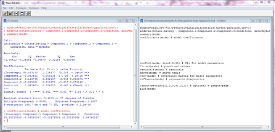
Figure 2 shows R’s built-in graphical user interface (GUI), which consists of an interactive command-line area on the left and a script window on the right.

Figure 2
The GUI of R
The bulk of R’s extensive predictive functionality is available through packages submitted by the worldwide network of R users and developers to the CRAN. While packages on the CRAN are subject to some pre-submission review and testing, much of the functionality is largely user-tested, and fixes and enhancements are made by concerned power users rather than a formal development team. This results in relatively robust and reliable code for commonly-used algorithms, but potentially less reliable code for more obscure algorithms. As is common with open-source, user-developed software, no formal support is available.
In addition to being freely available and open source, the main benefit of R is the flexibility it provides; as it is a programming language, a skilled programmer can implement virtually any algorithm in R. R was a natural choice for SAP to select as an engine for Predictive Analysis; not only does it complement the in-memory HANA architecture, but also, as an open-source programming language, R will never be acquired by a competitor, thus never cutting off SAP’s access to the critical predictive engine. However, since R is free, SAP must add significant value beyond the available R algorithms to justify the licensing cost of Predictive Analysis.
As of release 1.0.9, Predictive Analysis uses 13 R algorithms in each of the offline and HANA online modes, and R algorithms are the sole source for most of the offline algorithms (e.g., association, classification, clustering, and decision trees). The R algorithms are available in offline mode once the user installs R on a local machine, including the required packages that Predictive Analysis uses. R algorithms are also intended to be used for online HANA processing, for which R is installed on a separate host that interacts with the HANA server directly. Predictive Analysis is compatible with any version of R 2.11 or higher; the latest available version of R is 3.0.1.
The HANA Predictive Analysis Library
The HANA Predictive Analysis Library (PAL) is a set of predictive algorithms in the HANA Application Function Library (AFL). It was developed specifically so that HANA can execute complex predictive algorithms by maximizing database processing rather than bringing all the data to the application server.
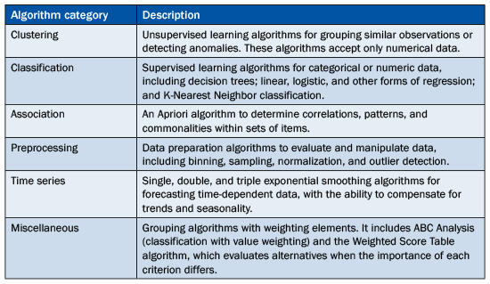
The HANA PAL is available with any HANA implementation — Service Pack (SP) 05 or higher — after installation of the AFL. The PAL makes predictive functions available that can be called from SQLScript code on HANA. As of SP05 (March 2013), six categories of algorithms are available in the PAL with 23 total algorithms represented. The six categories are described in
Table 1.

Table 1
Algorithm categories in the HANA PAL
While the PAL is available on any HANA implementation, without Predictive Analysis, PAL algorithms are called exclusively through scripting in HANA Studio and require a technical programmer or statistician to use. Additionally, any visualization or evaluation of the model fit requires significant coding and exporting results to a visualization tool for reporting.
Predictive Analysis Local Algorithms
While Predictive Analysis relies most heavily on the R predictive engine and the PAL in HANA online mode, seven algorithms are available for local (offline) processing that are not sourced from R. Most of these duplicate available local, R-based algorithms (triple exponential smoothing time series models and five varieties of regression), but these local algorithms are the only source for the outlier detection algorithms. The local predictive algorithms allow Predictive Analysis to have somewhat similar functionality in offline mode that the PAL provides in the HANA online mode, but the bulk of the predictive modeling functionality is available via the R predictive algorithms in offline mode.
A Detailed Look at SAP Predictive Analysis
SAP Predictive Analysis is built on the same codeline as SAP Lumira, encompasses all the functionality of Lumira, and adds a predictive tool. The UI for both Lumira and Predictive Analysis is being updated frequently as new features are added, and is likely to undergo significant changes as the visualization rendering is transferred from Java to HTML5.
Upon opening a Predictive Analysis document, three views are available from a selection bar at the top:
- The Prepare pane includes all the Lumira visualization and data manipulation functionality
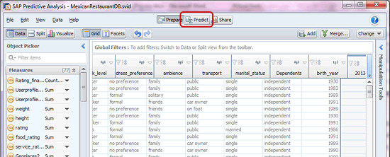
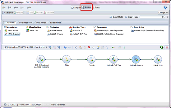
- The Predict pane (Figure 3) holds all the Predictive Analysis functionality, including data preparation, modeling, and data writer tools (and is not available when viewed in a Lumira-only installation)
- The Share pane, which allows users of Predictive Analysis and Lumira to share documents and objects (this pane appears in both Lumira and Predictive Analysis)

Figure 3
Predictive Analysis features appear on the Predict pane
Let’s break down the functions of Predictive Analysis and provide more details for the following areas:
- Lumira functionality
- Predictive Analysis architecture
- Predictive Analysis functionality
Lumira Functionality
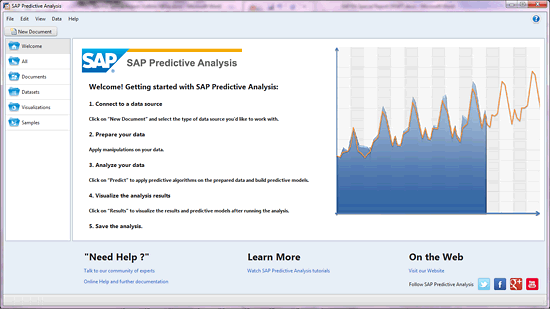
Upon opening Lumira or Predictive Analysis, users are greeted by a welcome screen in which they can create a new document or open previously created documents, datasets, and visualizations (
Figure 4).

Figure 4
The home page of Predictive Analysis
To create a new document, click the New Document button.
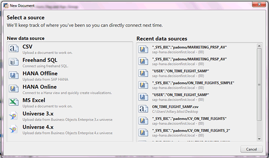
Figure 5 lists the selections for data sources that are available for the new document.

Figure 5
Select a source for a new document
Predictive Analysis operates in two modes: online with data on HANA or offline with downloaded data. Clicking the HANA online data source link activates the HANA online processing mode; all other selections on the screen transfer the selected data to the user’s local machine and activate offline mode. The mode determines whether data manipulation features are enabled and which predictive algorithms are available.
As of this writing in June 2013, Predictive Analysis does not officially support connections to universes (OLAP or relational) connected directly to an SAP NetWeaver BW source, but this is an often-requested feature among current and prospective users. The only supported scenarios for viewing SAP NetWeaver BW data in Predictive Analysis include the following:
- Run SAP NetWeaver BW on HANA and create a calculation view based on an InfoProvider from BW
- Import a DataStore object (DSO) or BW query snapshots as HANA analytic views or flat files, which can then be sources for Lumira or Predictive Analysis (HANA online or offline modes)
In the absence of BW on HANA, the user can create a relational universe on top of the DSO, which can be a source for a Predictive Analysis offline mode document. While many SAP community members have reported successful test cases using this workaround, SAP does not officially support this solution.
The fastest way to get data into Predictive Analysis is to import a plain text or Microsoft Excel file. Like many other modeling tools, Predictive Analysis can also pull data directly from a variety of databases via ODBC connections. With the appropriate data access driver, Predictive Analysis can access data on any of the following platforms via freehand SQL queries:
- Microsoft SQL Server (2005, 2008, and 2012 versions)
- Oracle (versions 10 and 11)
- Sybase IQ (version 15)
- Teradata (versions 12 and 13)
- IBM DB2 (versions 9 and 10)
- IMB Netezza (ask your Netezza administrator for assistance on the correct version)
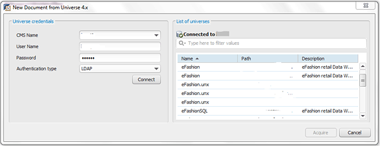
In addition to downloading data via freehand SQL, users can extract data from existing SAP BusinessObjects universes (either *.unv or *.unx files) to extract data rather than re-building this infrastructure in a file extract or freehand SQL Query. After you select one of the universe data sources and navigate to the BusinessObjects server, Predictive Analysis shows the list of universes available (
Figure 6).

Figure 6
A Predictive Analysis connection to a BusinessObjects universe server
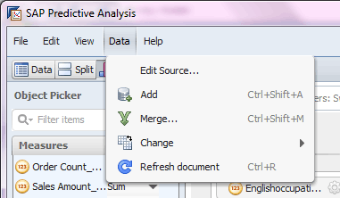
After choosing a universe, the user can select the fields from available universe objects and measures to include in the analysis set. Once the fields for the universe query are selected, the user can preview the data to make a final inspection of the fields that will download. The universe query is saved within the Predictive Analysis document. You can refresh the data downloaded to Predictive Analysis clicking Data > Refresh document (
Figure 7) or alter it to include fewer columns by clicking Data > Edit Source. You can add attributes by clicking Data > Add and creating a new universe query or adding an alternate source (which can be any other offline source, such as a text file or freehand SQL statement) and then clicking Data > Merge.

Figure 7
Options under the Data menu
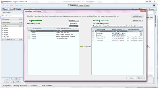
Once a new dataset has been added to the document, you can merge the new and old datasets together on a common field or leave them as separate analysis sets (
Figure 8).

Figure 8
Merging data sets in Predictive Analysis
The biggest advantage of Predictive Analysis’s direct integration with universes and databases is that the data extract definition (i.e., the universe query or freehand SQL statement) is stored within the Predictive Analysis document, and an updated dataset can be accessed on demand. When manual queries are written to extract data to text files for importing into modeling software, the field calculations and selection criteria might be lost or not well documented and, thus, be very time consuming to re-create.
Predictive Analysis works well with HANA. See the sidebar, “Accessing Data Online with HANA,” for further details.
Accessing Data Online with HANA
In addition to downloading data and running locally on the client machine, Predictive Analysis can also work in conjunction with a HANA server and Linux host to run the PAL and R algorithms. You can access HANA online data from HANA tables, calculation views, and analytic views. In HANA online mode, there are no data manipulation features such as those available in Predictive Analysis, but you can still use all the visualization tools.
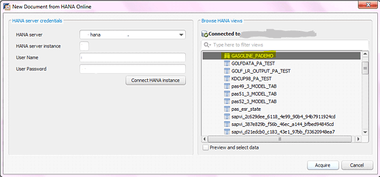
In addition, accessing data that resides in HANA increases the capacity of Predictive Analysis, as it is no longer limited by the processing power of the client machine. After specifying the HANA connection information, the user can select from a list of all HANA objects available (
Figure A). Once the source object is selected, the user can further trim the analysis set by taking the follow actions:
- Mark the box for Preview and select data
- Choose only a subset of the fields to be available in Predictive Analysis

Figure A
Navigate HANA objects in Predictive Analysis
For organizations with existing HANA infrastructure (e.g., attribute views, calculation views, analytical views, and other database elements), attributes and metrics used in existing BI documents can be examined directly through Predictive Analysis rather than being recreated via freehand SQL or a manual extract. Even when new HANA information views must be created for modeling, these objects are persistent on the HANA server, allowing the Predictive Analysis data to refresh at the click of a button. The modeling datasets and metrics are also available to other users to analyze in BI documents, reports, dashboards, and visualization tools.
Data Manipulation
Once the data has been loaded from one or more sources, data manipulation components allow analysts to modify and create data elements quickly. Grouping and transforming data is particularly important to the model building process. Many modeling tools allow for minimal data manipulation, requiring the analyst to generate an entirely new modeling extract to change age groupings, for example. Predictive Analysis facilitates calculations and manipulations on existing columns and adding further lookup data sources to avoid the need to manipulate data outside the tool.
Note
Documents accessing HANA online data sources have data manipulation, enrichment, addition, and merge features disabled. All data manipulation for HANA online data must be performed in the information views sourced for the Predictive Analysis document.
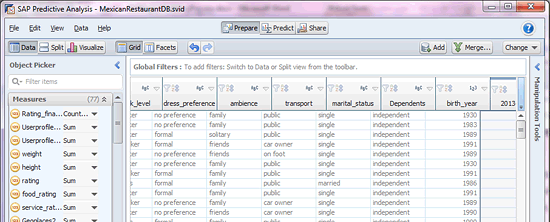
For example, the dataset in
Figure 9 has a birth year column, but age is more appropriate as a modeling variable because it is not time dependent. A model can predict the behavior of 20-year-old people today, next year, and five years from now, and will always be predicting the behavior of incoming 20-year-old people based on the experience data. Therefore, age must be calculated before modeling.

Figure 9
Preparation of a modeling dataset with the birth_year column
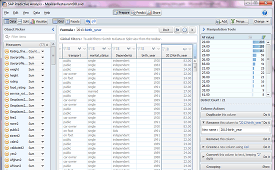
In the Prepare pane, select the birth_year column and click the Manipulation Tools banner along the right edge of the screen to expand it. In the resulting pane, click the Rename heading and type 2013-birth_year in the New name field (
Figure 10). Click the Do it link, and a new column with the age appears, along with a quick summary of the data.

Figure 10
Create a column showing age
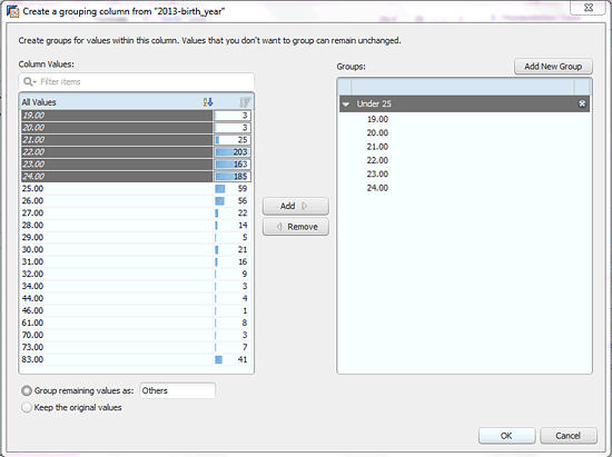
Because more than half of the observations are 22-, 23-, or 24-year-old people, age groups may be more appropriate. Click the Grouping heading in Manipulation Tools and create new groups for Under 25 and 25 and Over. Select the desired ages to be included from the left pane shown in
Figure 11 and click the Add button for each group. Doing so creates a grouping hierarchy on the right pane.

Figure 11
Creating age variable groupings in Predictive Analysis
The new grouped age variable is now available for modeling, visualization, and exploration on either the Prepare or Predict panes. The Manipulation Tools menu has automated solutions for changing case of variables, replacing values, and trimming leading and trailing spaces. A lengthy list of additional functions is available in the function menu, including date manipulation functions, string processing, numeric functions, and logical operators. Applying functions in the function bar creates a new column in the data, while selecting from the Manipulation Tools window implements changes to the existing data.
Data Enrichment
Once data is imported into Predictive Analysis, the software automatically detects potential enrichments to the attribute fields. Enrichments provide additional functionality for specific types of attributes. For example, date fields enriched as time hierarchies have automatic subtotals for year, quarter, month, and other intervals. Predictive Analysis can enrich data in one of three ways:
- Geographic hierarchy
- Time hierarchy
- Semantic enrichment (create a measure)
Note
For HANA online data, only geographic hierarchies can be enriched within Predictive Analysis. Measures and time hierarchies must be defined in the HANA information views prior to import into Predictive Analysis. While measures are not required for using predictive algorithms, they are required for creating any visualizations in Predictive Analysis.
Upon importing data into Predictive Analysis, the tool automatically detects any possible enrichments, with results shown at the bottom of the Object Picker toolbar on the left side of the Prepare pane (
Figure 12).

Figure 12
Predictive Analysis indicates it has detected possible enrichments
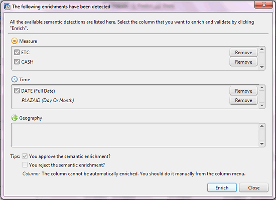
Clicking the Enrich All button automatically accepts and implements all auto-detected enrichments. The user should review the suggested enrichments by clicking the Show button, which provides a list of the detected enrichments (
Figure 13), allowing the user to remove enrichments that were not accurately detected by Predictive Analysis, such as numeric attributes that should not be measures. Then click the Enrich button to carry out the remaining enrichments.

Figure 13
A list of detected enrichments
Predictive Analysis automatically detects numeric fields to be measures (including key fields and numeric attributes) and partial date hierarchies (day or month). It also detects any fields with a date format as a date hierarchy.
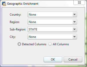
The geographic hierarchy enrichment allows a user to assign an attribute column to represent one of four geographic divisions: country, region, sub-region, and city (
Figure 14). Alternatively, users can define a geographic hierarchy based on latitude and longitude. Right-click any field in the attribute list to manually select an enrichment for that field, which then opens the screen in
Figure 14.

Figure 14
Geographic enrichment options
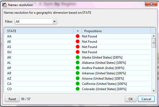
Once the geographic hierarchy has been defined, Predictive Analysis automatically detects the appropriate geographic object based on text and verifies this with the user, prioritizing elements that cannot be matched or were inconclusively matched to the geographical reference shipped with Lumira (
Figure 15).

Figure 15
Inconclusively matched elements
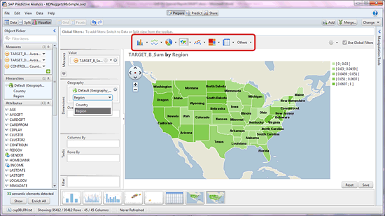
After the user accepts or updates the automatically detected geography by selecting an alternative geographic assignment for any unmatched or inconclusive assignments, one or more geographic elements are available for inclusion in charts or geographic charts. Predictive Analysis includes the following chart types in the geographic visualizations menu, indicated by the red oval in
Figure 16: choropleth chart (i.e., a map with different shades based on measurements), bubble chart, and pie chart.

Figure 16
A choropleth chart showing states in different shades
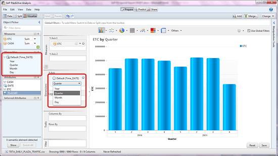
Similarly, you can construct time hierarchies from one or more fields. For example, a full date field automatically creates a year-quarter-month-day hierarchy, and you can assign individual fields for any of those values. Once the time hierarchy is created, the higher-level categories automatically appear on the Object Picker (
Figure 17) and are available for selection into visualizations. Once you select a time element as an X-axis dimension, you can access other time elements via a drop-down menu within the existing time dimension element rather than having to select a different dimension element for other date segments.

Figure 17
Date hierarchy in the Object Picker and as an X-axis dimension element
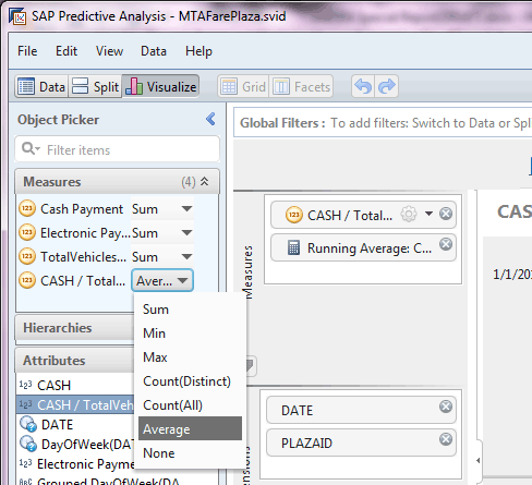
With offline data, users can create measures whenever necessary by right-clicking an attribute and clicking Create a measure, or by selecting the drop-down list on the measure and changing the aggregation method (
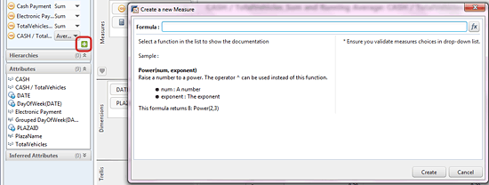
Figure 18). With version 1.0.9 of Predictive Analysis, users can also create calculated measures (
Figure 19) by clicking the Create a new Measure button and using the Lumira formula library.

Figure 18
Change the aggregation method for a measure

Figure 19
Create a calculated measure
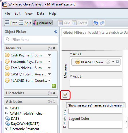
Predictive Analysis does not automatically create any measures in the document, so users must determine and create measures within the document or in the sourced HANA information view for HANA online datasets. Without one or more measures in the document, it is impossible to create any visualization of the data, so users should create at least a count measure to visualize the data. The count measure allows the user to view frequencies of records within each dimension. To create a count measure in offline mode, right-click any attribute, click Create a Measure, and select the count aggregation method. Also, the 1.0.9 release offers the ability to use measures as dimensions by clicking the Show measures’ names as a dimension icon

(
Figure 20). This allows users to visualize the same variable as an aggregation and a categorical variable, and can facilitate visualizations in which both the X and Y axes are measures, such as scatter plots.

Figure 20
Click the Show measures’ names as a dimension icon
Data Visualization
Predictive Analysis has an easy-to-use data discovery tool available under the Prepare pane. The point-and-click interface lets users perform pre-modeling data exploration tasks more quickly than writing code or summarizing the data and exporting the results to a visual tool, such as Excel.
Several types of charts are available by clicking the Visualize mode on the Prepare pane, including bar charts, line charts, pie charts, geographic charts, tree and heat maps, tabular view, and others (
Figure 21).

Figure 21
Chart options available in the Visualize mode
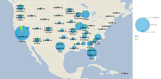
Many of these visualization charts can display many data dimensions in a single graphic. For example, in the geographic pie chart in
Figure 22, the data’s observations (solicitations for donation to a charitable organization) are geographically skewed, with populous states such as New York, Virginia, Pennsylvania, and Ohio barely represented. You can also see that the response rate (the green slice of the pie) varies significantly among states, suggesting that the state dimension may be a valuable predictor.

Figure 22
A geographic pie chart
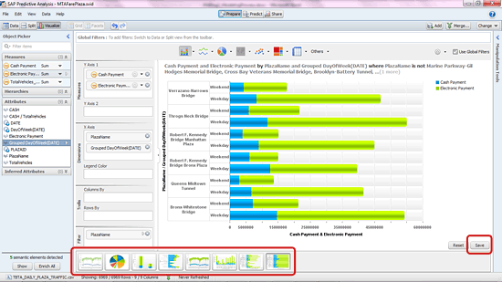
Switching between visualization types (e.g., from bar chart to pie chart to time series chart) takes only a few clicks using the icons at the top of the screen (
Figure 23). This encourages investigation into patterns in the data. Predictive Analysis also allows users to store visualizations with interesting insights by clicking the Save button in the lower right of the screen, highlighted in red in
Figure 23; these saved visualizations are kept in a library, shown across the bottom of the Prepare pane in the red rectangle.

Figure 23
A saved visualization library
You can share these saved visualizations, along with the modified datasets, by clicking the Share tab at the top. Once the Share pane is open (
Figure 24), you can send items from the document to others via email, upload items to SAP StreamWork, publish them to BusinessObjects Explorer, export them as a text files, or write them to a HANA table.

Figure 24
Options to share saved visualizations
Predictive Analysis Architecture
Predictive Analysis is installed and run locally on the client machine. As of release 1.0.9, Predictive Analysis could only run on Windows 7 (both 32- and 64-bit clients are available). Release 1.0.10 brought compatibility with Windows 8, but Windows Server and Mac OS remain unsupported. While it is likely that SAP will extend functionality to other Windows versions, there has been no indication that Mac systems will be supported.
Predictive Analysis has a small library of built-in predictive functions for linear regression, time series analysis, and outlier detection. The software largely relies on the local R, HANA PAL, and HANA-R predictive libraries for most of its predictive functionality.
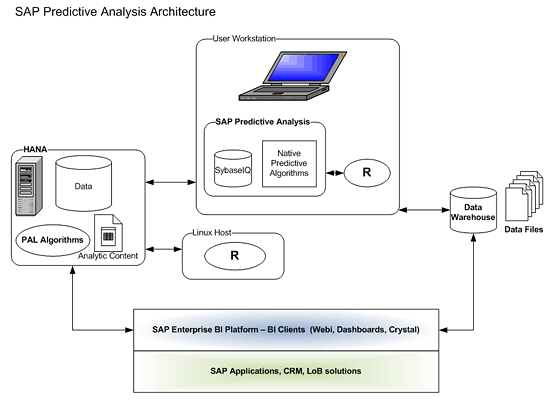
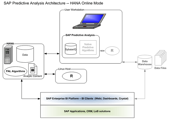
Figure 25 shows the full Predictive Analysis architecture and interaction with data sources.

Figure 25
Predictive Analysis architecture
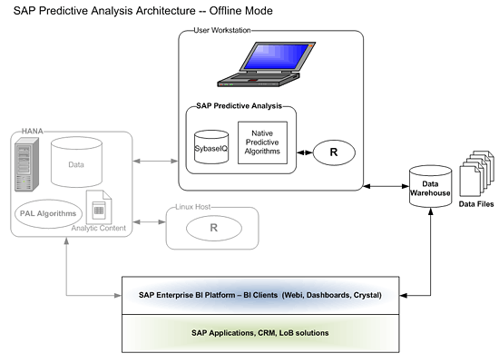
Predictive Analysis operates in two modes:
- HANA online mode, in which data is stored on HANA and predictive algorithms are run on either HANA or an affiliated R Linux host
- Offline mode, in which data from a flat file or database is downloaded to the user’s workstation and processed using only the client system resources
Each Predictive Analysis document operates only in HANA online or offline mode and cannot be changed. In HANA online mode, local R algorithms are not available, and in offline mode, the HANA PAL and HANA R algorithms are not available, even if the data was originally sourced from HANA.
HANA Online Mode
In HANA online mode, the data remains on the HANA system, and all visualization queries, predictive algorithms, and resulting data are also stored on HANA. This enables larger volumes of data to be processed through predictive algorithms than would be possible on the desktop client alone.
Figure 26 shows the architecture of Predictive Analysis for HANA online data sources.

Figure 26
The architecture of Predictive Analysis in HANA online mode
HANA supports the R scripting language and SQLScript language. R is supported on HANA by including an R client in the HANA calculation engine. The R client on HANA connects to an Rserve instance on an affiliated Linux host.
Rserve is a TCP/IP server that supports remote connection, authentication, and file transfer and allows access to any functionality of R to be integrated into other applications. Rserve is called by an R client, versions of which are available for Java, C++, R, Python, .NET/CLI, C#, and Ruby. Rserve is supported on most operating systems. However, the HANA-R implementation currently only officially supports R running on a SUSE Linux host.
Because the R algorithms are running on a separate machine, there is some cost to marshaling data between systems; however, since this process does not involve writing data to disk, the effect on predictive algorithm runtime is minimal. Additionally, the HANA calculation engine’s matrix primitives are relatively close in structure to Rserve’s data frame structure, so the marshaling cost of moving the data between the HANA calculation engine and Rserve is limited primarily by network bandwidth.
In an optimal implementation, the HANA and Rserve boxes are co-located with sufficient bandwidth to support large datasets. The data transfer between R and HANA is in a binary form, which further increases speed and reduces the quantity of data transferred across the network.
Each concurrent R call requires a separate connection to the R host, so if there is a high number of Predictive Analysis users frequently running lengthy modeling routines, HANA administrators may need to configure multiple ports or have multiple R hosts available to ensure high availability.
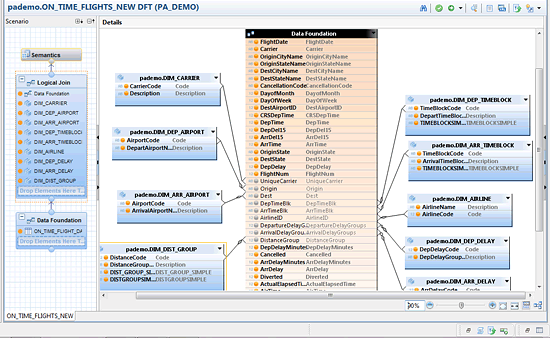
In HANA online mode, there is little data manipulation functionality available in Predictive Analysis. Therefore, all data modeling, calculations, cleansing, and value grouping must be done in HANA. The example in
Figure 27 shows an analytic view used for Predictive Analysis; the value lookups into the attribute views must be performed in HANA and cannot be imported as separate text files and joined within Predictive Analysis.

Figure 27
An analytic view for Predictive Analysis
These limits may require a Predictive Analysis user to be well versed in one of the following:
- An extract, transform, and load (ETL) tool to build datasets
- HANA data modeling
Alternatively, the user could partner with a team member who can implement these changes during the modeling process. Although it may require more work up front, building the modeling datasets in HANA is a best practice, since this ensures that the modeling dataset definition is preserved within HANA and updated data is available instantly. This also facilitates scoring of the model later within the HANA database, as the fields required for the model are already defined within the HANA database. One possible implementation scenario is to perform initial exploratory analysis and data manipulation in offline mode, in which the business user can manipulate and re-group variables, and then implement the final required variables in a HANA analytic view once the model has been approved.
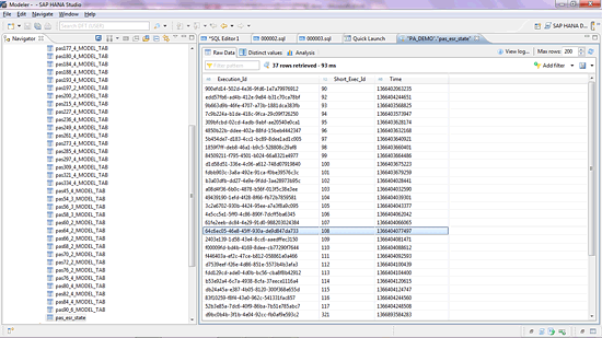
As a part of running the predictive algorithms in HANA online mode, Predictive Analysis stores records of the predictive modules called in the user’s schema on HANA.
Figure 28 shows tables that have been created by running predictive algorithms in a HANA online Predictive Analysis document. The last table in the list, pas_esr_state, shows a list of all executions for which the logged-in user was associated with that schema and the time (GMT) in milliseconds since January 1, 1970, that each one was executed. This approach may be useful for monitoring use of the Predictive Analysis tool on HANA by each user; assuming most of these require R algorithms, this also helps monitor the use of the Rserve box.

Figure 28
Tables created by running predictive algorithms in HANA online
The rest of the tables include result information for the actual models run in Predictive Analysis. Each of the pas##_X_MODEL_TAB tables holds the printed output displayed in the text results window in Predictive Analysis and the P
redictive Model Markup Language (PMML) model output. In addition to tables like the ones above, several stored procedures are created with each run of Predictive Analysis, and column stores are also created for saved visualizations and other intermediary data manipulation steps.
This content is not particularly useful to users, but it does appear to persist significantly after the Predictive Analysis session is closed, even if the document it was created under is not saved. While these items are typically quite small and shouldn’t take up significant space in HANA, the volume of content that can be created through normal use of Predictive Analysis could quickly make it difficult to navigate any HANA schemas used with Predictive Analysis. Therefore, HANA administration teams must be aware that this content is being created and periodically clean out some or all of it in any user schemas that log into Predictive Analysis.
Tip!
For HANA online data, only geographic hierarchies can be enriched within Predictive Analysis. Measures and time hierarchies must be defined in the HANA information views prior to import into Predictive Analysis. While measures are not required for using predictive algorithms, they are required for creating any visualizations in Predictive Analysis.
One additional consideration for the HANA online mode is that a HANA user accessing Predictive Analysis must have sufficient permissions to select from, execute, and write any data or analytic content that is used for prediction and visualization. A best practice is to create a predictive user security role on HANA and ensure that role has sufficient access to complete modeling tasks, but limit predictive users to select access only in schemas that should not be altered. Predictive users must also have the system privilege to CREATE R SCRIPT and the AFL__SYS_AFL_AFLPAL_EXECUTE role to execute HANA PAL scripts, and user _SYS_REPO must have SELECT privileges with the ability to grant to others on the predictive user’s named schema.
With the introduction of version 1.0.10, Predictive Analysis began calling PAL functions using a new API, which requires the creation of the AFL_WRAPPER_GENERATOR(SYSTEM) procedure and granting any Predictive Analysis user accounts execute privilege on this procedure. This new API supports only a limited range of field types; all datasets used for PAL algorithms under 1.0.10 must have only Integer, Double, VarChar, or nVarChar data types in independent columns. The presence of any other field types causes a live cache error when the PAL algorithm is called.
Offline Mode
Predictive Analysis is less complex in offline mode. Data is imported via the configured database connectors via freehand SQL or a flat text file.
Figure 29 shows the system interaction for Predictive Analysis operating in offline mode.

Figure 29
The architecture of Predictive Analysis in offline mode
The imported data is saved in the Predictive Analysis document within Sybase IQ. Therefore, when a Predictive Analysis document is shared among users of Lumira and Predictive Analysis, the shared document is fully functional and includes all the original data. While the document is open, the data is stored in memory on the user’s workstation; for this reason, very large datasets can cause slow performance, not only during prediction, but also for visualization.
Once the data is imported and manipulated in Predictive Analysis, most of the predictive algorithms on the Predict pane are actually calling functions in the locally installed version of R. All the data processing in the local R engine is performed on the user’s workstation and is limited by the dataset size in R and the available memory in R and on the workstation.
Installation Notes
Installing the local version of Predictive Analysis is a simple installation of an executable file. Once this is installed, R must also be installed locally on the user’s workstation. SAP has included a built-in R installation utility available under the File menu within Predictive Analysis, which enables R algorithms and starts a download of the R application and required packages, as shown in
Figure 30. If this download does not work, the user must manually install the R application (version 2.15.1 or later) and the required R packages and then point Predictive Analysis to the directory in which R is installed.

Figure 30
The R Installation and Configuration utility
To access the HANA PAL through Predictive Analysis, you need up upgrade HANA to SP05 or higher and install the AFLs. In addition, you need to enable the scripting server, per
SAP Note 1650957. More information on the installation of the AFL is available in
SAP HANA Installation Guide with Unified Installer for SP05 section 3.8: Installing Application Function Libraries (AFLs) on a SAP HANA System.
R is neither supported nor shipped by SAP because R is open source and protected under a general public license. The HANA administrative team or R host administrator must install and configure Java, R, and the required R packages for Predictive Analysis on the R host, and configure and enable the R client in the HANA calculation engine. For further details, refer to the
SAP HANA R Integration Guide. If the Linux host is running SUSE with an active support agreement, you can download and install R and Rserve via the update repository. In this situation, there is no need to compile the R code.
Additional information and test cases for the installation process are available in this installation guide posted on Decision First Technologies’
SAP BI Blog. Because Lumira and Predictive Analysis have been combined, a user can only have one of the two applications installed on a workstation at one time. Users with Lumira or a previous version of Visual Intelligence must uninstall the visualization-only version of the application before they can install Predictive Analysis.
Predictive Analysis Functionality
Most of the functionality unique to Predictive Analysis is found on the Predict pane (
Figure 31), which is only available to users who have licensed the Predictive Analysis version of the tool; otherwise, users see only the Prepare and Share panes that appear in Lumira.

Figure 31
The Predict pane
The Predictive Workflow
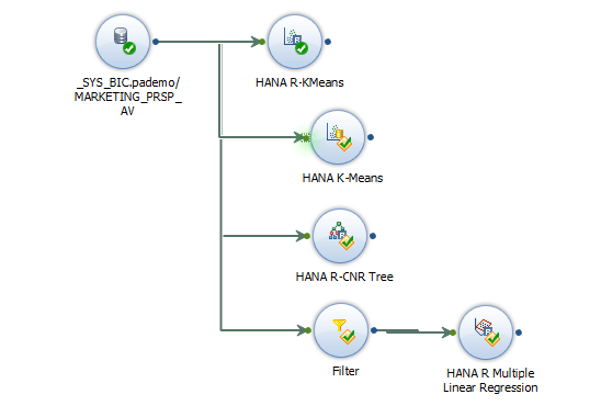
The Predict pane features a predictive workflow design area in the lower half of the screen, which allows users to string together data sources, data manipulation modules, algorithms, models, and data writers to build predictive analyses. These predictive workflows can be linear, like the example in
Figure 31, or branched to create separate analyses for comparison between alternatives or to run separate modules, like in the example in
Figure 32.

Figure 32
A branched predictive workflow
Branching the transforms allows only a portion of the analysis to run. Clicking the green arrow icon

above the predictive workflow runs the entire workflow. However, hovering over a module within the workflow and clicking the green-and-yellow arrow icon

(which also provides a message of Run Till Here) allows users to run only the predictive workflow steps prior to and including the selected step (
Figure 33). Doing so reduces runtime and processing resources and allows a user to verify that the intermediate steps provide the expected results prior to running the entire analysis.

Figure 33
Running a partial workflow
Predictive algorithms can also run sequentially, and you can use the results of one model as an input into a second modeling algorithm. In the example in
Figure 34, you can use the predicted customer cluster from the HANA R-KMeans algorithm as an input variable in the HANA R-CNR Tree model.

Figure 34
You can use the results of one model as an input into another model
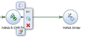
Hovering over a module in the predictive workflow reveals several options (
Figure 35). From top clockwise, they are:
- Rename

- Run Till Here, which I discussed earlier
- View Results (this becomes available once the module is executed)

- Delete

- Configure Properties


Figure 35
Options within a workflow
You must configure properties for all elements in a predictive workflow except the source object prior to running. When a module is first brought into a workflow, such as the HANA Writer element in
Figure 35, the empty diamond icon within the element

indicates that it is not configured. The configuration check prior to execution only ensures that required fields are populated, and is not a guarantee that the predictive workflow will execute without errors.
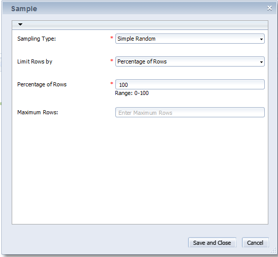
Clicking the Configure Properties button opens the object’s configuration window. Only fields in the configuration window marked with a red asterisk must be entered. For example, in the Sample module configuration, three of the four inputs are required (
Figure 36). Once the object’s properties are configured, like the HANA R-CNR Tree module on the left in
Figure 35, a green check mark icon

appears on the object.

Figure 36
The configure properties window for Sample object
Data Preparation Modules
In addition to the data manipulation functionality in the Prepare panel, there are several modeling-related data preparation modules available in the algorithm library, which appears in the top half of the Predict pane.
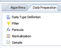
Figure 37 shows the available data preparation functions available in offline mode. In HANA online mode, only the Filter and Sample tools are available.

Figure 37
Data preparation functions in offline mode
Let’s look at these data preparation functions further. Filter and Sample are used to reduce records or fields (e.g., randomly, systematically, or logically) going into the modeling transforms. Filter can remove records that should not be considered in a model (e.g., outliers or missing data).
Data Type Definition and Formula allow for manipulation of the input or output data. Data Type Definition changes the name of a column or the format of a date field. Formula allows for basic manipulation of the data and aggregate calculation.
Formula includes date manipulation formulas, string manipulation formulas, and logical expressions. There are also several aggregating mathematical functions that calculate the maximum, minimum, sum, average, and count within the entire column. These functions cannot be nested within one another in the same function block, but the same result can be achieved with sequential function blocks. The data manipulation formulas @REPLACE and @BLANK can replace specific or blank values. This duplicates functionality that exists already in the Prepare pane, but explicitly programming these rules as formulas means that the manipulation rules are documented and a part of the predictive workflow. Thus, when new data files in the old format are imported into the project, the rules can be automatically applied rather than going back through the manipulation steps in the Prepare pane.
The Normalization algorithm is a data transformation commonly used prior to modeling. Normalization adjusts the scale of the variables. There are a variety of methods of normalization, but the most popular are min-max normalization, which scales values between 0 and 1 by subtracting the minimum value and dividing by the range of the dataset, and standardization or z-score normalization, which re-centers the values and divides by the variance to make the data comparable to a standard normal (N(0,1)) distribution.
Predictive Algorithms
The library of predictive algorithms is found in the top half of the Predict pane. The list of included algorithms available in Predictive Analysis is one aspect of the tool that is changing quickly. With every release, SAP adds algorithms. As an example,
Figure 38 shows the full list of algorithms available in offline mode as of release 1.0.10, while
Figure 39 shows a
lgorithms available in online mode for the same version.

Figure 38
Predictive algorithms available in offline mode in version 1.0.10

Figure 39
Predictive algorithms available in online mode in version 1.0.10
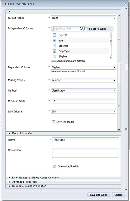
Within each predictive algorithm, there are typically one or two main fields that must be configured by clicking the Configure Properties button prior to running. Most models require one or more predictors (often called independent columns) to be selected from the available fields in the document, and the supervised learning algorithms (including decision trees and regression models) further require the results or dependent variable to be defined (
Figure 40).

Figure 40
Predictors for the HANA R-CNR Tree
Most of the other options default to commonly selected values; for example, the clustering algorithm defaults to five clusters, but this may not be appropriate depending on the dimensionality of the input data and the business needs of the organization. Users should carefully review settings for things like Output Mode, Missing Values, and Method options, and understand the effect of keeping the default settings. Some information on the details of each configuration option is found in the Predictive Analysis documentation (follow menu path Help > Help), but users may need to have a statistical background, such as understanding the meaning and effect of changing prior probabilities or fitting methodologies, in order to fully understand all settings.
There are additional options that users may want to consider changing as well. Examples include renaming output columns, saving the predictive model, and updating optional model properties that may help the model conform to more realistic business expectations (e.g., limiting the complexity of a decision tree).
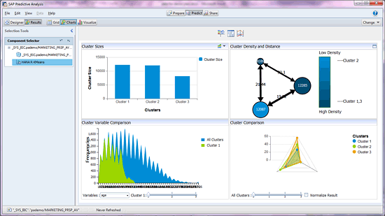
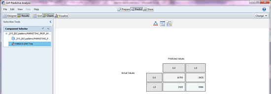
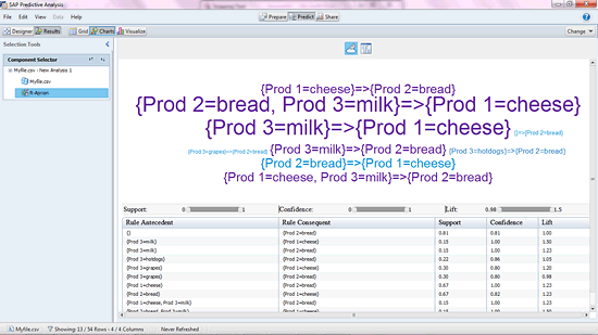
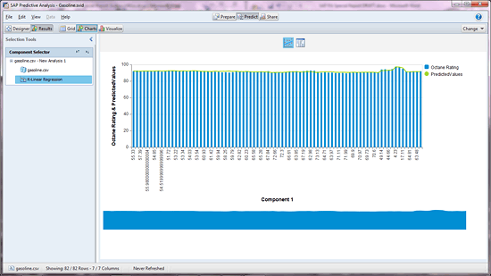
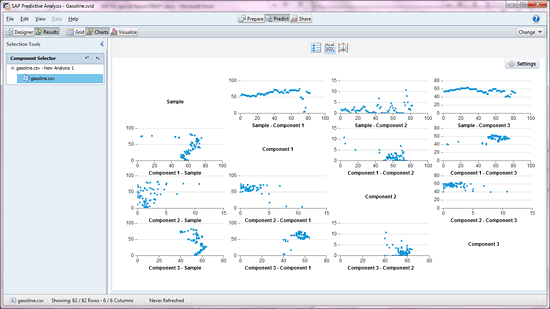
One of the most important features of Predictive Analysis is the automated result visualization and diagnostic reporting. With Lumira’s visualization tools, Predictive Analysis offers some impressive model visualizations. The quality, usefulness, and readability of visualizations vary greatly by algorithm. Visualization samples for algorithms with graphical output are included in
Figures 41 through
45.

Figure 41
The results visualization for an R-KMeans clustering algorithm

Figure 42
The results visualization for an R-CNR decision tree algorithm

Figure 43
The results visualization for an R-Apriori association algorithm

Figure 44
The results visualization for an R-Linear Regression algorithm

Figure 45
The results visualization for automated dataset statistics
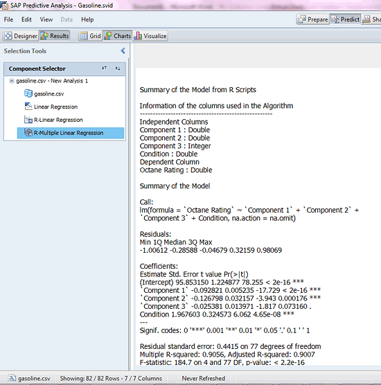
In addition to the graphical visualizations, typically the standard algorithm output from the R algorithm is printed in the text results output visualization. While the R summary output often has valuable information — such as coefficient values, fit statistics, and predictor significance — the output may be illegible due to poor text formatting. An example of the text output for multiple linear regression is shown in
Figure 46. This text output information is valuable not only to data scientists evaluating the fit of models, but also to the business units that must implement predictive models in other systems.

Figure 46
The text output for multiple linear regression
A point to be aware of in Predictive Analysis: The resulting visualizations for some algorithms are limited in the number of observations that can be displayed. For example, the regression algorithm visualization displays each observation compared to the predicted value. For a small dataset, this is valuable, but for a dataset with several thousand observations, Predictive Analysis cannot display any graphical output. In this case, the user is left with only the text output and predicted values in the resulting dataset to determine the fit and significance of the model. Typical visualizations for regression output include outlier distributions, residual analysis, and one-way correlations and relationships between predictors. Currently, none of these default visualizations are automatically available for regression models in Predictive Analysis, although I expect SAP to address this issue in future enhancements.
Exporting Predictive Data
Let’s start by reviewing how to export predictive data in offline mode. Datasets and predictive workflow results can be written to a database system via a JDBC connection, which requires some configuration within the predictive workflow. The user must configure connection options shown in
Figure 47.

Figure 47
JDBC Writer module options for exporting predictive workflow data back to a database
Alternatively, the predictive workflow can write to delimited text files. Text files from Predictive Analysis can be picked up by an ETL process and loaded into the database.
In HANA online mode, the only output source to include in a predictive workflow is a HANA writer module, which writes the output dataset to a table in HANA. This has the option of overwriting an existing table, which replaces the named HANA table (if it exists) with the output dataset from Predictive Analysis.
Exporting Predictive Models
Once models are developed within Predictive Analysis, users can export the model scoring algorithm in either *.SVID or *.PMML formats. The SVID file format is unique to Predictive Analysis and allows users to exchange models and import previously built models into new Predictive Analysis documents.
PMML is an XML-based markup language that was developed by data mining industry groups to provide an industry-standard way to represent predictive models. PMML defines modeling and limited preprocessing structures for the most common predictive models, including clustering, association, regression, time series, and trees.
Most predictive modeling tools can export PMML modeling formats; however, it is somewhat uncommon for databases or applications to be able to consume PMML models natively. There are commercially available scoring engines that you can deploy in the cloud to score PMML models via a Web service, on a batch basis, or even using plug-ins to Excel. Alternatively, there are database plug-ins for several common databases — including Teradata, EMC Greenplum, Netezza, and Sybase — which allow scoring models to be called as a function once PMML models have been imported.
One of the benefits of integrating a PMML plug-in into an existing database is that the database can then consume predictive models from virtually any predictive modeling tool, and organizations can use multiple tools or switch tools with little effect on the deployment timeline.
You can use these same methods to integrate predictive algorithms with other applications. While it is unlikely that applications will automatically be equipped to accept PMML model objects, incorporating these objects into a Web service or creating a stored procedure to run the algorithm equation allows a model algorithm to be called by many applications within an organization. Alternatively, the algorithm equation could be programmed directly into the application for calculation. Select the implementation method based on the algorithm complexity.
The Future for Predictive Analysis
While Predictive Analysis introduces new functionality packaged with attractive visuals, SAP has acknowledged that there are many enhancements required to bring Predictive Analysis functionally up to par with other popular statistical tools. The following sections outline likely enhancements to Predictive Analysis based on SAP’s published roadmap and logical product enhancements based on existing infrastructure and the competitive marketplace.
Architecture
SAP has invested significantly to prepare the infrastructure for Predictive Analysis: converting the codeline to align with Lumira, committing to the R modeling engine, and integrating the Rserve and PAL functionality from HANA. Therefore, from an architecture perspective, there is not much chance of significant change, including the introduction of other predictive engines. In addition, SAP has stated that Predictive Analysis was engineered with consideration for HANA and in-memory processing and has significant dependence on the HANA PAL, so it is unlikely that in-database predictive functionality will extend for any other non-HANA database solutions. However, there may be additional databases supported for accessing and writing data using JDBC connections.
While the architecture of Predictive Analysis is unlikely to change drastically, SAP has discussed enhancements to the operation system requirements; version 1.0.10 (May 2013) introduced compatibility with Windows 8, and in future 2013 releases Predictive Analysis will likely run on Windows Server operating systems. In addition, more management and automation tools for Predictive Analysis are expected, such as the ability to schedule model runs automatically.
A scenario that SAP has said is unlikely to occur is the ability to use an external R host in offline mode — in other words, rather than pointing Predictive Analysis to a local installation of R, using a higher-caliber server R instance for running predictive algorithms, even when not connected to HANA. The lack of processing integration databases other than HANA and ability to use an external R host means that organizations that do not have HANA are limited to the processing power of the local client machine when using Predictive Analysis.
Data Preparation and Predictive Algorithms
Over the next few releases, SAP is expected to add the remaining HANA PAL algorithms that are not yet available in Predictive Analysis. This includes both predictive and preparation algorithms, perhaps most notably the popular CHAID decision tree algorithm and logistic regression, which is useful for predicting the probability that something will occur, such as making a transaction, defecting from a subscription, or responding to a marketing solicitation. Also, because SAP has thus far kept the HANA online and offline functionality consistent, it is probable that these same algorithms will be implemented in offline mode, either as proprietary Predictive Analysis functions, or perhaps more likely through the integration of R algorithms equivalent to the PAL algorithms.
In addition, the PAL itself is expanding, with new algorithms expected through 2013, including neural networks, support vector machines, additional clustering algorithms, and advanced tools such as the following:
- Bagging, which is used with another predictive algorithm, such as neural networks or decision trees, to improve the accuracy and stability of the model by fitting multiple models with random sub-samples of the training data
- Boosting, which attempts to create a single, highly accurate predictor by using a weighting methodology to combine multiple weak predictors
- Cross validation, which creates multiple models from various samples of the available training data and averages the different models to produce a final prediction
- ARIMA (Autoregressive Integrated Moving Average) models, which are fitted to time-series data to better understand trends and improve forecasts
- Monte Carlo simulation, which obtains predictions based on simulations run many times, rather than attempting to force the problem into a deterministic algorithm or for situations in which it is impossible to obtain a closed-form expression
At some point after these new algorithms are added to the PAL, they will likely also be included in Predictive Analysis, continuing the goal of parity between the PAL and Predictive Analysis algorithms.
Beyond the new algorithm modules that are programmed for use, SAP is going to open up the ability to run any R algorithm from Predictive Analysis with the introduction of a code window that will let users configure modules for any R package by writing R code to call the function. Users could also use this code-based tool to create modules to run any algorithm they program in R, and are not limited to those available in packages. Using the custom R code functionality would require that users have any packages they are planning to use installed on the R instance accessed by Predictive Analysis. Programming custom R modules requires a technically savvy user, but once modules are programmed, they could be shared and reused by multiple users.
Visualizations and Model Evaluation
Users can expect further enhancements to the post-modeling visualization and evaluation tools in Predictive Analysis. Some modeling algorithms have useful and informative visualizations, but other algorithms have minimal, if any, diagnostics included in the automated output. In addition to visualizing the results of the model, modelers must complete a series of diagnostic tests during the model evaluation and selection process to ensure that the model is a good fit and statistically sound.
Users should expect to see high-quality visualizations of model fit for many algorithms over the next several releases. Although SAP has not shared specifics around which visualizations they intend to provide, some standard diagnostic tools would include lift charts, residual plots and analysis, influential point and outlier analyses, correlation and multicollinearity testing, and goodness-of-fit tests. There are many packages available in R for graphical model diagnostics, so it is possible that these could be implemented either as R algorithms or natively within Predictive Analysis.
On the technical side, within the next few revisions, SAP will introduce a new HTML5 user interface (UI) for Predictive Analysis, which will render all visualizations in HTML5. In addition, visualizations and model results will be able to be saved within the *.SVID Predictive Analysis document. In revisions 1.0.10 and prior, model results and visualizations are not saved when a document closes, and models have to be re-run to inspect the results. Finally, SAP has indicated there will be more efficient support for visualizing large datasets; currently the limits for time series and regression charts are fewer than 10,000 observations.
Model Deployment
While Predictive Analysis already supports exporting scoring models as *.SVID or *.PMML documents, SAP plans to make models even easier to implement in any database by supporting the export of model rules as SQL procedures. This may first be extended only to PAL algorithms. This would likely eliminate the need for third-party database plug-ins to consume PMML models.
SAP has also announced that a near-future enhancement for HANA (via the PAL) will include functionality to import PMML models, allowing Predictive Analysis-created models to be imported into HANA quickly and easily.
In addition to making scoring algorithms available as SQL procedures, SAP has suggested that the scoring algorithms could be exported as stub or pseudo code that could easily be adapted to any language and integrated in either a database or front-end application.
SAP has also said that future releases of Predictive Analysis will include model version management features and comparison, which allow organizations to monitor and document models throughout the modeling life cycle.
SDK and Strategic Integration
One of the strategic plans for Predictive Analysis and Lumira is to integrate the predictive and visualization features with SAP line-of-business applications. This may be accomplished through the Predictive Analysis software development kit (SDK) that is planned for the future. Although these plans have not been shared in detail, information released in the past indicates that the SDK would allow developers to create and modify algorithm logic within created components, use visualizations of Predictive Analysis in external applications, and write their own visualizations.
One aspect of the SDK is the generic R package support and the creation of components or modules using any R package or user algorithm. However, there is the potential that the SDK could expand to embedding predictive functionality and visualizations within external applications, making the functionality available to a much wider audience. It is likely that SAP will integrate Predictive Analysis features directly into many of its line-of-business applications (e.g., SAP Customer Relationship Management), and you could perform additional integration if SAP makes the SDK available.
Another strategic plan that SAP has announced is the intent to include predefined analytic dialogs within the tool for common business needs in select vertical markets. This is a long-range planned enhancement, so no specifics have been announced, but this would most likely include guided, wizard-like configuration processes for common analyses such as customer segmentation, churn analysis, market-based analysis, or next-most likely purchase rules. This is a strategic move to make the tool more accessible to non-data scientists and further expedite the predictive process.
SAP is pursuing both ends of the technical spectrum for Predictive Analysis, extending both the technical features with the generic R code support, which can be used by coders and data scientists to run customized and unsupported algorithms, and also facilitating use by the less-technical business users through more automated visualizations and predictive dialogs.

Decision First Technologies
Decision First Technologies (DFT) is a professional services company specializing in delivering end-to-end business intelligence solutions to its customers. An SAP gold-channel partner and six-time SAP BusinessObjects Partner of the Year, DFT resells and offers certified consulting, training and technical support for all analytics as well as database and technology products in the SAP BusinessObjects portfolio. DFT’s comprehensive BI solutions allow users to access, analyze, and share information stored in multiple data sources, including SAP and non-SAP environments. The company’s data warehousing practice designs and implements enterprise solutions utilizing SAP Business Warehouse, appliances such as SAP HANA or traditional relational database technologies. With more than 10 years of experience, DFT has helped hundreds of companies make better business decisions, dramatically reducing costs, increasing revenues, and boosting profits. For more information on Decision First, visit
https://www.decisionfirst.com/ or follow on Twitter
@DecisionFirst.
If you have comments about this article or publication, or would like to submit an article idea, please contact the
editor.

Hillary Bliss
Hillary Bliss is the analytics practice lead at Decision First Technologies and specializes in data warehouse design, ETL development, statistical analysis, and predictive modeling. She works with clients and vendors to integrate business analysis and predictive modeling solutions into the organizational data warehouse and business intelligence environments based on their specific operational and strategic business needs. She has a master’s degree in statistics and an MBA from Georgia Tech. You can follow here on Twitter
@HillaryBlissDFT.
Hillary will be presenting at the upcoming SAPinsider Customer Engagement & Commerce 2017 conference, June 14-16, 2017, in Amsterdam. For information on the event, click
here.
You may contact the author at
Hillary.Bliss@decisionfirst.com.
If you have comments about this article or publication, or would like to submit an article idea, please contact the
editor.

