Learn how to carry out causal analysis in SAP Advanced Planning and Optimization (SAP APO) when demand is correlated with some known and measureable factor (demand is a function of some variables). Understand how regression is used to find correlations between a single dependent variable (y) and one or more independent variables (x1, x2…xn) and how it is carried out.
Key Concept
Forecasting is a process involving qualitative and quantitative techniques to predict future demand values. In forecasting techniques, regression analysis is used for prediction and forecasting. It basically helps to identify the relationship between an independent variable such as price on a dependent variable such as demand. Simple linear regression is a function of a single independent variable while multiple linear regression (MLR) is function of more than one independent variable.
Forecasting is part of the Demand Planning (DP) and management process in SAP Advanced Planning and Optimization (SAP APO). The system reads historical data and calculates the corresponding values that it proposes as the future data. Causal models can be very useful when you can determine (and measure) the underlying factors that drive the demand of your product. Causal analysis can be carried out not only on a product but on any characteristic as per business scenario.
You can use causal models in scenarios in which you have independent variables, such as price, that have some influence on a dependent variable, such as sales quantity. With this information, you can set up the system to make sales react in a certain way when you change the price in the future. Multiple linear regression (MLR) is a form of causal analysis model. It enables you to analyze the relationship between a single dependent variable and several independent variables. I focus on how to use causal models in forecasting demand in SAP APO along with understanding the underlying mathematical model.
Overview of Forecasting and Causal Analysis
Forecasting is one of the components of an organization’s DP and management processes. It basically helps to answer questions such as what the expected demand is for a product in the next six to 12 months. Forecasting methodologies can be divided into two modes – subjective and objective. Subjective methodologies are more qualitative and are heavily dependent on judgment and educated guesses/surveys. Objective methodologies, on the other hand, are more quantitative and rely heavily on past data. Within objective methodologies two widely used techniques are time series and causal models.
Time series models are used where one believes by studying patterns in the past data, future demand can be predicted. Components of time series models are level, trend, seasonality, error, and cyclical. Causal models are used where demand is dependent on some known factors. For example, temperature can be one of the major factors that can influence the sales of ice cream or the rate of unemployment can be studied to correlate with number of occurrences of crime in a society.
Figure 1 shows a high-level classification of forecasting techniques and commonly used methods.

Figure 1
Classification of forecasting techniques
Note
A naïve forecast is a basic forecast method in which the past period’s actual value is used as the forecast for the next month without any adjustments.
To use causal analysis techniques within SAP APO, you need to complete following steps:
1. Set up SCM master data in SAP APO for product locations.
2. Set up and configure DP objects such as:
- Storage bucket profile
- Planning bucket profile
- Master planning object structure (MPOS)
- Planning area
- Characteristic value combination (CVC)
- Time series objects
- Planning book and data view
- Maintaining a forecast profile
- Loading time series data in the planning book
- Executing MLR
- Interpreting the results
Note
I assume that the reader knows how to set up master data in SAP APO and how to configure and navigate in basic DP objects. For this article, I focus on important configurations specific to forecasting and causal analysis and also show the structure of related DP objects. For the example discussed in this article, I have created a location with the name PLANT1 and location type 1001(Plant) in SAP APO. I have created a finished good product with the name FG01 at PLANT1 in SAP APO. In this article, I am creating a forecast for FG01 using different business scenarios. In step 1, setting up product locations in SAP APO is optional and not a mandatory step to carry out forecasting.
Planning Area
Planning area defines the area in which most of the planning activities take place. It groups together both characteristics and key figures under a single domain. A planning area is created via transaction /SAPAPO/MSDP_ADMIN. It contains three key figures: Forecast and two additional key figures, Future5 and Future6, as shown in Figure 2. The two future key figures (Future5 and Future6) are used to show the modeling of independent variables in the business scenario context later in the article, while the Forecast key figure is the dependent variable.
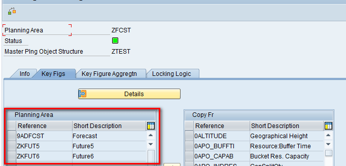
Figure 2
Planning Area
Planning Book
A planning book, which describes the layout of the interactive planning screen, is created via transaction /SAPAPO/SDP8B. I have created planning book ZFCST based on Planning Area ZFCST. While creating a planning book, you need to activate the multiple linear regression view by selecting the corresponding check box in order to use causal analysis in SAP APO as shown in Figure 3.

Figure 3
Planning book with MLR activated
All three key figures present in the Planning Area are assigned to the planning book in transaction /SAPAPO/SDP8B as shown in Figure 4.

Figure 4
Key figures assigned to the planning book
Regression and Mathematical Models Used in Regression
Regression models are used to predict dependent variables given a set of known independent variables. The model essentially tries to define a linear relationship that describes the behavior of a dependent variable given the behavior of independent variables. It is represented as:
Y = b0 + b1xi + b2xi + . . . for i = 1, 2…n
Putting the values i = 1, 2 in the equation results in the following equation:
Y = b0 + b1x1 + b2x2
In the above equation:
- x1, x2 = independent variables (by setting i = 1, 2 in the equation you get x1, x2, and so on.)
- b0 = constant
- b1, b2 = coefficients or weights
Simple Linear Regression Model
In the simple linear regression model, the relationship is defined in terms of a linear model. You have only one independent variable, so the regression equation would be Y = b0 + b1x1.
This simple example is useful in describing the model. Suppose that Table 1 shows the daily demand of a plant over a period of 10 days.
| Day |
Demand(y) |
| 1 |
10 |
| 2 |
13 |
| 3 |
12 |
| 4 |
18 |
| 5 |
21 |
| 6 |
19 |
| 7 |
25 |
| 8 |
22 |
| 9 |
25 |
| 10 |
27 |
Table 1
Demand of a sample plant over 10 days
The tabular data is presented as a scattered plot in Figure 5.
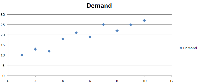
Figure 5
Scattered plot of daily demand of plant
With the above data, if you want to predict the demand for next five days using linear regression, then solving the model would give the following equation:
Y (Demand) = 1.8545x + 9 (how values are calculated is explained in a later section)
Here x = the dependent variable, which is the number of days.
So, demand for Day 11 = 1.8545 * 11 + 9 = 29 (Approx.). Similarly, you can calculate demands for other days by substituting the day in place of variable x as in the following equation:
Demand for Day 12 = 1.8545*12 + 9 = 31 (Approx.) and so on.
(Approx. is used because the results are rounded off to nearest whole digit number.)
How a Regression Model Calculates Values
A regression model basically tries to minimize residual or error terms. For example, suppose in the above example, the actual demand for day 11 = 32 while the forecast value was 29.
So, error term (e) = Actual – Forecasted = 32 – 29 = 3
In the same way the model also internally tries to minimize the error terms:
Error term (e) = Y (Actual) – Y (Forecasted)
= Y (Actual) - b0 - b1xi - b2xi for i = 1,2,..n
Therefore, you need to find the value of b that minimizes the error term. SAP APO uses ordinary least squares (OLS) regression to find the optimal value of b that minimizes the error term.
Mathematically, the equation in Figure 6 is used and a partial derivative is calculated to find the first order optimality condition with respect to each variable.

Figure 6
Minimizing error terms in OLS regression

Figure 7
Values of b1 and b0 in the regression model
In Figure 7 the new terms are y (bar) and x (bar), both of which are averages of y and averages of x, respectively.
Calculating the Regression Model Equation
Using the formulas in Figure 7, you can calculate values of b1 and b0 and put in the regression equation to calculate the value of dependent demand (Y). There are two options for calculating the values of b1 and b0, manually in Excel or using the LINEST function in Excel.
1. Calculating the Values of b1 and b0 Manually in Excel
You can calculate the values of b1 and b0 using the formulas in Figure 7 and the data shown in Table 1 via Microsoft Excel by calculating the values of different terms and putting in the formulas, respectively. Table 2 shows the calculations carried out based on the formulas in Figure 7. You can see values of b1 and b0 = 1.8545 and 9, respectively.
|
Day |
Demand(y)
|
y-y(avg.)
|
x-x(avg.)
|
x-x(avg.)^2
|
x-x(avg.)*y-y(avg.)
|
|
1 |
10 |
-9.2
|
-4.5
|
20.25 |
41.4
|
| |
2 |
13 |
-6.2
|
-3.5
|
12.25
|
21.7
|
| |
3 |
12 |
-7.2
|
-2.5
|
6.25
|
18
|
| |
4 |
18 |
-1.2
|
-1.5
|
2.25
|
1.8
|
| |
5 |
21 |
1.8
|
-0.5
|
0.25
|
-0.9
|
| |
6 |
19 |
-0.2
|
0.5
|
0.25
|
-0.1
|
| |
7 |
25 |
5.8
|
1.5
|
2.25
|
8.7
|
| |
8 |
22 |
2.8
|
2.5
|
6.25
|
7
|
| |
9 |
25 |
5.8
|
3.5
|
12.25
|
20.3
|
| |
10 |
27 |
7.8
|
4.5
|
20.25
|
35.1
|
| Sum |
|
|
|
|
82.5
|
153 |
| Average of x |
5.5 |
|
|
|
|
|
| Average of y |
19.2 |
|
|
|
|
|
| |
|
|
|
|
|
|
| b1 |
1.854545 |
|
|
|
|
|
| b0 |
9 |
|
|
|
|
|
Table 2
Calculating values manually in Excel
Putting the values of b1 and b0 in the equation, you get:
Y (Demand) = 1.8545x + 9
2. Using the LINEST Function in Excel to Calculate the Values of b1 and b0
You saw that you can calculate the values of b1 and b0 in the above step manually. However, that calculation method is cumbersome, so instead you can use the LINEST function that is available in Microsoft Excel. LINEST is basically an array function that receives and returns data to multiple cells. It is shown as:
LINEST(known_y's, known_x's, constant, statistics).
In the above function, y and x are independent and dependent variables, respectively. Constant and statistics are always 1 and 1.
Using the LINEST function in Excel gives output in the format shown in Table 3.
| b1 |
b0 |
| sb1 |
sb0 |
| R2 |
se |
| F |
df |
| SSR |
SSE |
Table 3
Output format of the LINEST function
Following are the definitions of terms in Table 3:
- sb0 = standard error of intercept
- sb1 = standard error of slope
- se = standard error of estimate
- R2 = coefficient of determination
- df = degrees of freedom
- SSR = sum of squares of regression
- SSE = sum of squares of the error
R2, which is the coefficient of determination, is used to validate the model. The range of R2 is between 0 and 1. It explains how good the model is in explaining the variability in the dependent variable. Generally if the value of R2 is greater than 0.70 then the model is considered to be good and is interpreted as the model explains 70 percent of variability. (Variability is the proportion of variance in the dependent variable that can be predicted from the independent variable.)
Continuing with the same example as in Table 1, you can use the LINEST function for the same data and Excel automatically calculates the values of b1 and b0 as shown in Figure 8.

Figure 8
Calculating values via the LINEST function in Excel
Putting the values of b1 and b0 in the equation, you get:
Y (Demand) = 1.8545x + 9
You can also note that value of b1 and b0 calculated by LINEST function is same as that calculated in step 1 (manually in Excel). Using this function is a smart and easy way to get the regression model equation instead of doing all the calculations.
The calculated regression equation is shown in Figure 9 by drawing the trend line on the scatter plot obtained in Figure 5 via Excel.

Figure 9
Trend line on scatter plot
Multiple Linear Regression Model
In contrast to the simple linear regression model, the only difference here would be the presence of more than one independent variable. Therefore, the regression equation would be:
Y = b0 + b1x1 + b2x2 (for two independent variables)
Y = b0 + b1x1 + b2x2 +b3x3 (for three independent variables) and so on.
Note
Simple linear regression always has time as the independent variable, whereas in multiple linear regression, you can have more than one independent variable that generally does not include time as a variable.
Carrying Out Linear Regression in SAP APO with One Independent Variable
In this section, I explain the concept of linear regression in SAP APO with one independent variable.
Business Scenario 1
Table 4 shows the monthly sales for a coffee shop distributed over time. The first column is the monthly time period. The second column is the average outside temperature for that month. The third column is the monthly demand for hot coffee. Based on the past data you would like to find out if monthly average temperature has any correlation with demand and you want to forecast the future demand with the average temperature there being 37, 39, and 36 as shown in Table 4.
Time period
|
Avg. outside temperature(x1)
|
Demand(y) |
| 1 |
37 |
3025 |
| 2 |
39 |
3136 |
| 3 |
46 |
3414 |
| 4 |
56 |
3502 |
| 5 |
67 |
3736 |
| 6 |
77 |
3661 |
| 7 |
82 |
3553 |
| 8 |
80
|
3691 |
| 9 |
73 |
3474 |
| 10 |
62 |
3876 |
| 11 |
52 |
3865 |
| 12 |
42 |
3967 |
| 13 |
37 |
3596 |
| 14 |
39 |
4345 |
| 15 |
46 |
4413 |
| 16 |
56 |
4086 |
| 17 |
67 |
4377 |
| 18 |
77 |
4220 |
| 19 |
82 |
4238 |
| 20 |
80 |
4007 |
| 21 |
73 |
4086 |
| 22 |
62 |
4536 |
| 23 |
52 |
4291 |
| 24 |
42 |
4427 |
| 25 |
37 |
? |
| 26 |
39 |
? |
| 27 |
36 |
? |
Table 4
Business scenario 1 data — demand for hot coffee in coffee shop
In the given scenario, you have one independent variable (i.e., avg. outside temperature), so the equation of linear regression to forecast the demand would be:
Y (Demand) = b0 + b1x1
Forecast Profiles
To create the forecast profile, execute transaction /SAPAPO/MC96B. In the next screen, give the name of planning area (e.g., ZFCST). Click the MLR Profile tab as shown in Figure 10.

Figure 10
Maintain the forecast profile in the Master Prfl. tab
In the MLR Profile tab, enter the name of Profile (MLR), Description (MLR), and MLR Method (Standard MLR Forecasting). In the scenario in this article, Forecast is the dependent key figure, so enter the Key Figure name 9ADFCST and Version 000. Then click the Key Fig. button as highlighted in Figure 11.
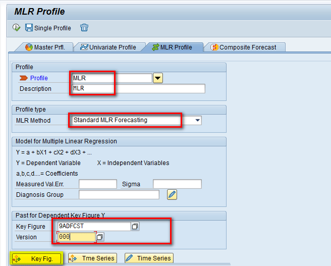
Figure 11
Maintain the forecast profile in the MLR Profile tab
In the pop-up screen, select the check box for the Future5 key figure and then click the enter icon (the green check mark) highlighted in Figure 12. Note the given business scenario has only one independent variable (i.e., avg. temperature), so I select only one key figure.

Figure 12
Assign an independent key figure to the MLR profile
In the same screen, enter the version for Key Figure Version 000 and then click the Single Profile button shown in Figure 13.

Figure 13
Enter values in the MLR Profile tab
In the same screen click the execute icon to assign the MLR Profile to the main master profile. A message appears at the bottom of the screen as shown in Figure 14.
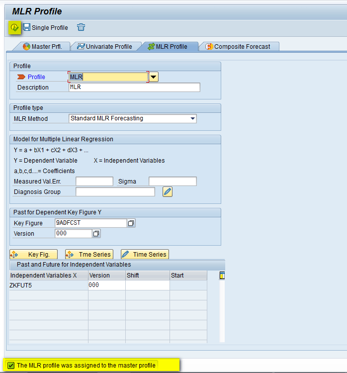
Figure 14
MLR profile assigned to the main master profile
In the Master Prfl. tab, enter the name (New Master Profile), the Forecast Key Figure (9ADFCST), Period Indicator (M for months), Forecast Horizon (January to March 2016), and the History Horizon (January 2014 through December 2015). Select the Multiple Linear Regression check box and enter the name of MLR profile created (MLR). Click the save icon highlighted in Figure 15.
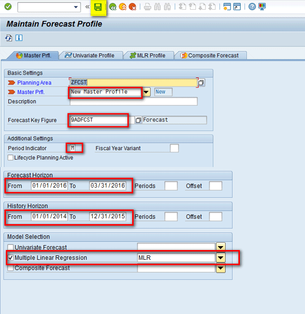
Figure 15
Enter values in the master profile
Data Entry in the Planning Book
After creating the forecast profile in the above step, you need to enter the data in the planning book. To enter the data as per Table 4 in the planning book, enter transaction /SAPAPO/SDP94. In the given scenario, Data for Demand is entered in the Key Figure Forecast. The first row in Figures 16 and 17 shows data for demand (e.g., 3025 and 3136) and the name of the key figure is Forecast. Enter data for Avg. Temperature in Key figure Future5 as shown in Figures 16 and 17. After entering the data, select the MLR icon highlighted in Figure 17. (Figures 16 and 17 show sections of the same screen.) To enter the data for 24 months (i.e., Jan 2014 to Dec 2015) you need to just scroll across the same page and enter the data in different monthly periods as shown in both figures together.

Figure 16
Data entered in the planning book

Figure 17
MLR executed in the planning book
Execute MLR
After you click the icon highlighted in Figure 17, a pop-up screen appears (Figure 18). Enter the name of the Master Profile (New Master Profile) and then click the execute icon.

Figure 18
Execute MLR
In Figure 19, you can see that the model has forecasted the value for January through March 2016 as 3536, 3492, and 3557, respectively, as shown in Figure 19. Click the highlighted forecast comparison icon.
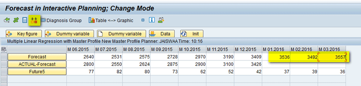
Figure 19
Forecasted values via MLR for business scenario 1
A new screen opens and you can see the value of R**2 as 0.83 (R**2 is same as R2, which is calculated by the LINEST function in Table 2) as shown in Figure 20. The value of 0.83 suggests that the model explains 83 percent variability in demand. As the value of R**2 is greater than 0.70, you can use the model. Since this opened in a new screen, after noting the value of R**2 you can close it.

Figure 20
R**2 in business scenario 1
In the same screen as in Figure 19, click the save icon and back icon as highlighted in Figure 21.

Figure 21
Save your data and exit from the planning book
Carrying Out Linear Regression in Microsoft Excel with One Independent Variable
Using the same data as in business scenario 1 data, you now model using the LINEST function in Excel and see if both of them give similar forecast values.
With the data in Table 4, use the LINEST function to generate values for b0, b1, and R**2 as highlighted in Figure 22.
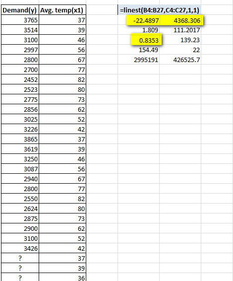
Figure 22
LINEST function on business scenario 1 data
The values of b0 and b1 = 4368.306 and -22.4897, respectively.
R2 = 0.8353 or 83% (Approx.), which is approximately equal to the R**2 value of 0.83 calculated by APO MLR model in Figure 20.
Forecasted Demand with avg. temp. 37 = 4368.306 – 22.4897*37 = 3536.186= 3536 (Approx.)
Forecasted Demand with avg. temp. 39 = 4368.306 – 22.4897*39 =3491.206 = 3492 (Approx.)
Forecasted Demand with avg. temp. 36 = 4368.306 – 22.4897*36 = 3558.676 = 3558 (Approx.)
You can see forecasted demands are 3536, 3492, and 3558 units, respectively, which are approximately the same as what was forecasted by the SAP APO MLR model in Figure 19. This shows how the underlying model being used in SAP APO and the LINEST function in Excel are the same.
Note
A negative value of b1 in the above result denotes that there is a negative correlation between average temperature and demand for hot coffee, which means that as the temperature goes down, the demand for hot coffee increases.
Carrying Out Linear Regression in SAP APO with Two Independent Variables
In this section, I extend the concept of linear regression to include multiple independent variables.
Business Scenario 2
Table 5 shows the monthly sales for a retail manufacturer shop that are distributed over time. The first column is the time period in months, the second column lists the selling price of the product for that month, the third column shows the amount spent on promotions in that month, and the fourth column shows the monthly demand of product. Based on the past data you want to understand if there is any correlation between demand, price, and promotion expense. You want to forecast the demand for time periods 13, 14, and 15 with target prices of 130, 150, and 155. The promotion expense is allocated as 6000, 5200, and 5800, respectively, as shown in Table 5.
Time period
|
Price(X1) |
Promotion(X2) |
Demand(Y) |
| 1 |
150 |
3000 |
12000 |
| 2 |
165 |
4000 |
13750 |
| 3 |
155 |
2500 |
11450 |
| 4 |
128 |
6500 |
17650 |
| 5 |
132 |
6000 |
16450 |
| 6 |
155 |
5500 |
14890 |
| 7 |
125 |
8000 |
19000 |
| 8 |
155 |
2700 |
11500 |
| 9 |
122 |
8250 |
19540 |
| 10 |
120 |
8500 |
19900 |
| 11 |
130 |
6200 |
17000 |
| 12 |
135 |
5800 |
16000 |
| 13 |
130 |
6000 |
? |
| 14 |
150 |
5200 |
? |
| 15 |
155 |
5600 |
? |
Table 5
Monthly sales for a retail manufacturer shop
In the given scenario, you have two independent variables (i.e., Price and Promotion), so you use multiple linear regression to forecast the demand. The equation here would be:
Y (Demand) = b0 + b1X1 + b2X2.
Forecast Profile
To change the forecast profile, execute transaction /SAPAPO/MC96B and go to the MLR Profile tab. In the Profile field, load the existing saved MLR profile (e.g., MLR) as highlighted in Figure 23. This automatically loads the other values of the fields shown in Figure 23 (e.g., MLR Method, Key Figure, and Version).

Figure 23
Load the existing MLR profile in the MLR Profile tab
In the given scenario you have two independent variables (i.e., price and promotion) so you also need to have two key figures defined. To do that, click the Key Fig. button shown in Figure 23.
In the pop-up screen that appears, select the check boxes for the Future5 and Future 6 key figures and then click the enter icon highlighted in Figure 24.

Figure 24
Assign two independent key figures to the MLR profile
In the MLR Profile screen (Figure 25), enter 000 in the Version field for Key Figure 9ADFCST. Click the save icon beside Single Profile, as shown in Figure 25, and then click the Master Prfl. tab.

Figure 25
Enter values in the MLR Profile tab
In the Master Prfl. tab, you need to change the Forecast Horizon and History Horizon time periods accordingly. Enter the History Horizon from January 2015 through December 2015 (12 months) and the Forecast Horizon from January through March 2016. Click the save icon as shown in Figure 26.

Figure 26
Enter values in the Master Prfl. tab
Data Entry in the Planning Book
You enter data in the planning book via transaction /SAPAPO/SDP8B as shown in Figure 27. Note that for January through March 2016, I entered values for the Future5 and Future6 key figures. The dependent key figure (i.e., Forecast) will be calculated by the model. After entering the data, select the MLR icon.
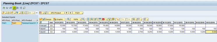
Figure 27
Data entered and MLR executed in the planning book
Execute MLR
After you click the MLR icon (Figure 27), a pop-up screen appears (Figure 28) in which you enter the name of the Master Profile (e.g., New Master Profile) and then click the execute icon.

Figure 28
Execute MLR
In the next screen, you can see that the model has forecasted the values for January through March 2016 as 16498, 15052, and 15470, respectively, as shown in Figure 29. Click the highlighted forecast comparison icon.

Figure 29
Forecasted values via MLR for business scenario 2
A new screen opens and you can see the value of R**2 as 1.00 (Figure 30). The value of 1.00 suggests that model explains almost 100 percent variability in demand and as the value of R**2 is greater than 0.70, you can use the model.

Figure 30
R**2 in business scenario 2
In the main screen, click the save icon and then the back icon as shown in Figure 31.
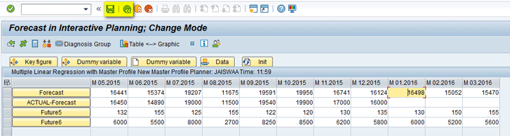
Figure 31
Save your data and exit the planning book
Carrying Out Linear Regression in Microsoft Excel with Two Independent Variables
Using the same data as in business scenario 2 data, you now model using the LINEST function in Excel and see if both of them give similar forecast values.
Using the data in Table 5, use the LINEST function. The values are generated for b0, b1, b2, and R**2 as highlighted in Figure 32.

Figure 32
LINEST function on business scenario 2 data
The values of b0, b1, and b2 = 11339.63, -20.305, and 1.2995, respectively.
R2 = 0.9909 or 99.9% (Approx.) which is approximately equal to R**2 value of 1.00 calculated by the APO MLR model in Figure 30.
Demand in Time period 13 with price of 130 and promotion of 6000 = 11339.63 - 20.305 * 130 + 1.2995*6000 = 16497.24398= 16498 (Approx.)
Demand in Time period 14 with price of 150 and promotion of 5200 = 11339.63 - 20.305 * 150 + 1.2995*5200 = 15051.49687= 15052 (Approx.)
Demand in Time period 15 with price of 155 and promotion of 5600 = 11339.63 - 20.305 * 155 + 1.2995*5600 = 15469.79055= 15470 (Approx.)
You can see that demands for time periods 13, 14, and 15 are 16498, 15052, and 15470 units, respectively, which are approximately the same as what was forecasted by the SAP APO MLR model in Figure 29. This shows how the underlying model being used in both SAP APO and LINEST function in Excel are the same.
Negative and positive values of b1 and b2 denote the corresponding correlation with demand. Since b1 is negative it means that as the price of the product goes down, its demand increases. Similarly a positive value of b2 denotes that as the amount spent in promotions goes up, the demand for products also increases.
Note
There are many other (and advanced) software packages that can do this and other statistical modeling you can use. However, they are both complex and expensive. In this article, I have demonstrated the regression concept using the LINEST function as it can be easily used in spreadsheets and is easy to understand and use.
Alok Jaiswal
Alok Jaiswal is a consultant at Infosys Limited.
He has more than six years of experience in IT and ERP consulting and in supply chain management (SCM). He has worked on various SAP Advanced Planning and Optimization (APO) modules such as Demand Planning (DP), Production Planning/Detailed Scheduling (PP/DS), Supply Network Planning (SNP), and Core Interface (CIF) at various stages of the project life cycle.
He is also an APICS-certified CSCP (Certified Supply Chain Planner) consultant, with exposure in functional areas of demand planning, lean management, value stream mapping, and inventory management across manufacturing, healthcare, and textile sectors.
If you have comments about this article or publication, or would like to submit an article idea, please contact the editor.