Buffer Profiles and Buffer Level Determination
My first article discussed the Demand Driven Planning logic in SAP ECC or SAP S/4HANA using SCM consulting solutions, which are small add-on tools that can be used in SAP to cover so called “white spots”. The second article focused on first step in Demand Driven Planning, which is Strategic Inventory Positioning, identified by the Demand Driven Institute, to detect which materials should be decoupled and which not. This article will focus on the second step, called Buffer Profiles and Buffer Level Determination.
For each decoupled material, buffer zones are calculated. Buffer levels are divided into four zones: green, yellow, red, and dark red. These color codes are based on the increasing urgency of the stock situation which are called buffer zones. Buffer zones are calculated dynamically using parameters such as average daily usage and decoupled lead time. These are defined below.
Red zone: The red zone represents the highest severity in the buffer and indicates low stock levels and the immediate need for replenishment. The buffer value at the top of the red zone is the safety buffer, which is the minimum recommended buffer level. The red zone can be further divided into red and dark red zones. The dark red zone represents the minimum safety buffer.
Yellow zone: The yellow zone represents medium severity in the stock buffer. This indicates that the stock levels are lower than their ideal value and replenishment is required. The cumulative sum of the quantities of the red and yellow zones results in the reorder point.
Green zone: The green zone represents the lowest severity in the stock buffer. If the available stock is within this zone, there should be enough stock to cover the current demand. The maximum stock is the cumulative sum of the quantities of the red, yellow, and green zones and represents the recommended maximum buffer level above which the stored stock level is considered to be excessive.
The size of each zone, and therefore the size of the total buffer is different for each material. These values are determined in the image below.
Buffer Zones in Demand-Driven Planning
Starting from the average daily usage, the individual zones are calculated as per the below:
Yellow Zone
Average Daily Usage x Decoupled Replenishment Lead Time
Red Zone
Yellow zone x Red replenishment lead time factor
Dark Red Zone
Red zone x variability factor
Green Zone
Maximum of
Yellow zone x replenishment lead time factor green
or
minimum lot size
or
Average daily usage x order interval
To avoid determining the buffer zones for each material manually, buffer profiles are defined and assigned to different material groups. Individual material characteristics are added to it. The buffer profiles and the individual material characteristics are used to calculate individual buffer levels for each material.
Buffer Profiles and Levels
The following parameters are used for buffer sizing and are different for each material, two of which are for the yellow zone and one for the green zone. First, the two formula parameters for the yellow zone must be determined:
- Average daily usage (ADU) Average Usage Demand – ADU)
- Decoupled replenishment lead time (DLT) Decoupled Lead Time - DLT)
- The minimum order quantity (MOQ) is used for the green zone.
Subsequently, materials are grouped according to specific characteristics and corresponding buffer profiles are assigned.
The average daily usage is calculated using transaction/SAPLOM/MRP. On the Data Basis tab page, the analysis period and the data source that are to be used as the basis for calculating the average daily usage need to be specified (as shown in the image).
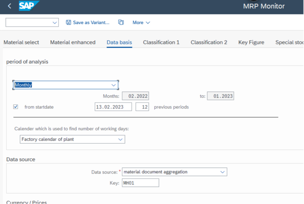
MRP Monitor: Data Basis for Calculating Average Daily Usage
The average daily usage can be calculated in three variants (as shown in the image below).
- Only based on consumption (past periods)
- Only based on forecast (future periods)
- Based on the combination of consumption and forecast (past and future periods)
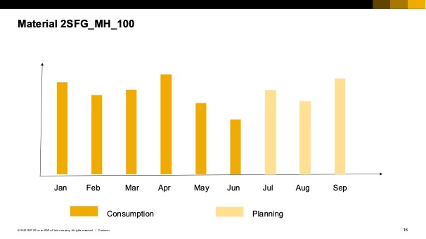
Period Selection for Calculating Average Daily Usage
The second formula parameter for yellow zone calculation is the decoupled replenishment lead time. This is calculated using the consulting solution replenishment lead time monitor and transaction /SAPLOM/RLT (as shown in image below).
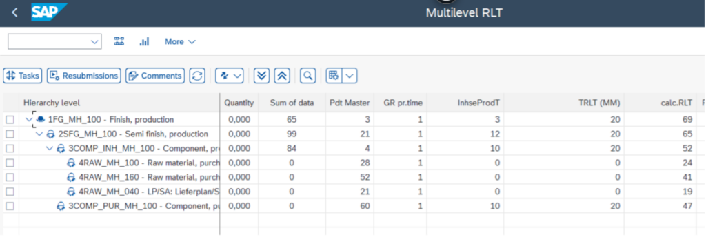
Calculation of the Decoupled Replenishment Lead Time for Material 2SFG_MH_100 in the Replenishment Lead Time Monitor
The decoupled replenishment lead time can now be updated in the material master, on the SCM CS 1 tab page in the corresponding field (as shown in image below).
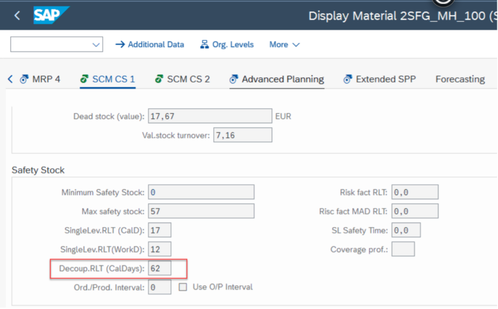
Material Master: SCM CS 1 View – Decoupled Replenishment Lead Time
Next, the minimum lot size which is another material attribute located in the material master on the MRP 1 tab is required (as shown as image below).

Material Master: MRP 1 View – Minimum Lot Size
To be able to calculate all zones, buffer profiles must be created and assigned to the materials.
Buffer Profiles
To create buffer profiles and assign them to materials, the materials are first grouped according to their characteristics. It is recommended that they are grouped according to the following criteria:
- Procurement type: in-house production (E), external procurement (F)
- Decoupled replenishment lead time: short (E), medium (F), or long (G.
- Supply and/or demand variability: low (x), medium (y), or high (z).
This is only a proposal since the profiles that are actually created should be defined on a company-specific basis. Based on the material classification and the procurement type, the three factors are assigned to the buffer profiles (as shown in Table 1).
- The replenishment lead time factor green (LFG)
- Red replenishment lead time factor (LFR)
- Variability factor Red (VF)
| Procurement Type |
EFG Classification |
XYZ Classification |
DLT
|
LFR
|
VF |
| E |
E |
X |
0.8 |
0.8 |
0.25 |
| E |
E |
Y |
0.8 |
0.8 |
0.5 |
| E |
E |
Z |
0.8 |
0.8 |
0.75 |
| E |
F |
X |
0.5 |
0.5 |
0.25 |
| E |
F |
Y |
0.5 |
0.5 |
0.5 |
| E |
F |
Z |
0.5 |
0.5 |
0.75 |
| E |
G |
X |
0.2 |
0.2 |
0.25 |
| E |
G |
Y |
0.2 |
0.2 |
0.5 |
| E |
G |
Z |
0.2 |
0.2 |
0.75 |
| F |
E |
X |
0.8 |
0.8 |
0.25 |
| F |
E |
Y |
0.8 |
0.8 |
0.5 |
| F |
E |
Z |
0.8 |
0.8 |
0.75 |
| F |
F |
X |
0.5 |
0.5 |
0.25 |
| F |
F |
Y |
0.5 |
0.5 |
0.5 |
| F |
F |
Z |
0.5 |
0.5 |
0.75 |
| F |
G |
X |
0.2 |
0.2 |
0.25 |
| F |
G |
Y |
0.2 |
0.2 |
0.5 |
| F |
G |
Z |
0.2 |
0.2 |
0.75 |
Buffer profiles in demand-driven planning
Longer green and red replenishment lead times result in shorter replenishment lead time factor. For example, 0.2 for long, 0.5 for medium, and 0.8 for short lead time.
For the variability factor, more variability leads to higher variability factor. For example, 0.25 for low, 0.5 for medium, and 0.75 for high variability.
Calculating Buffer Zones
To calculate the buffer zones, the average consumption is calculated over the total decoupled lead time (that is ADU x DLT). This value represents the yellow zone or consumption within the (decoupled) replenishment lead time.
The remaining zones are calculated as follows:
- Green zone: yellow zone x replenishment lead time factor green
- Exception: if the minimum order quantity is higher, use the minimum order quantity instead.
- Red zone: yellow zone x replenishment lead time factor red
- Dark red zone: red zone x variability factor
Then, starting from the dark red zone, the zones are added together:
- Top of Red zone (TOR): dark red zone + red zone
- Top of Yellow zone (TOY): red zone + yellow zone
- Top of Green Zone (TOG): Yellow Zone + Green Zone
Buffer zones can be calculated using the consulting solution Safety Stock and Buffer Simulation. To do this, call transaction /SAPLOM/SSS.
As an example, the zones have been calculated and shown in the image below.
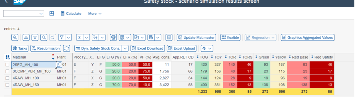
Buffer Calculation with the Safety Stock and Buffer Simulation Consulting Solution
The example of material 2SFG_MH_100 should be followed in detail (as shown in image below).
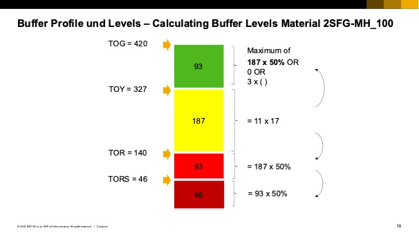
Buffer Calculation for Example Material 2SFG_MH_100
The average daily usage of three pieces within the decoupled replenishment lead time of 17 days results in a yellow zone of 187 pieces.
The red zone is calculated from the yellow zone (187) multiplied by the replenishment lead time factor for the red zone (50%), which results in 93 pieces. The dark red zone is calculated as 93 pieces (red zone) * variability factor (50%) = 46 pieces.
Dark red zone: 46 pieces = 46 Top of Red Safety (TORS)
+ red zone with 93 pieces = 140 Top of Red (TOR)
+ yellow zone with 187 pieces = 327 pieces Top of Yellow (TOY)
+ green zone with 93 pieces = 420 pieces Top of Green (TOG)
The buffers can be transferred to the material master, tab page SCM CS 2, using the Material Master Update button (as shown in image below).
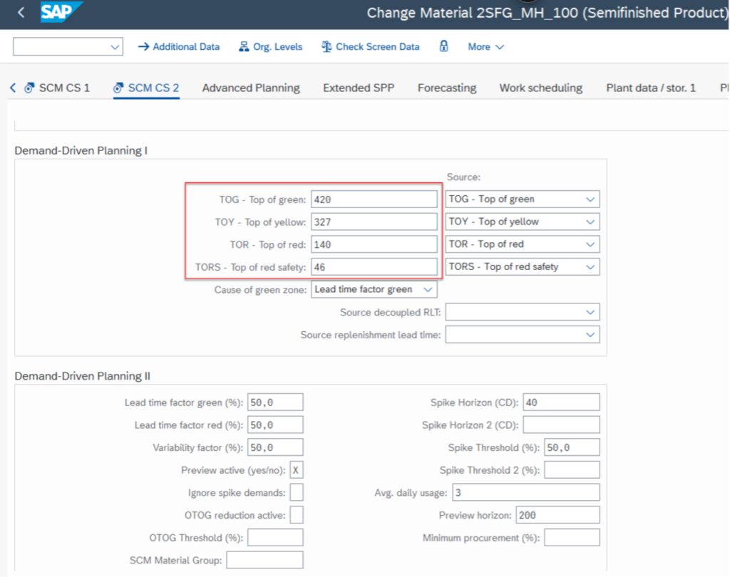
Material Master: SCM CS 2 View – Demand-Driven Buffer
After assigning the buffer profiles and calculation of buffer levels for all decoupled materials, the master data needs to be updated accordingly.
The next step is dynamic adjustments, which will be explained in the next article of the series. Click here for part three in the series.